Quicksort: Average case

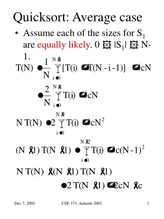
1. Quicksort: Average case • Assume each of the sizes for S1 are equally likely. 0  |S1|  N-1. CSE 373, Autumn 2001

2. Average case, continued divide equation by N(N+1) … loge (N+1) – 3/2 CSE 373, Autumn 2001

3. Selection • Find the kth smallest element in an array S. • quickselect(S, k): • If |S| = 1, then k=1 and return the element. • Pick a pivot v S. • Partition S – {v} into S1 and S2. • If k |S1|, then the kth smallest element must be in S1. Return quickselect(S1, k). • If k = 1 + |S1|, return the pivot v. • If k > 1 + |S1|, then the kth smallest element is in S2. Return quickselect(S2, k - |S1| - 1). CSE 373, Autumn 2001

4. Analysis of Quickselect average case: … = O(N) worst case: same as Quicksort,O(N2) CSE 373, Autumn 2001

5. A Lower Bound • information-theoretic lower bound for comparison-based sorting. a < b < c a < c < b b < a < c b < c < a c < a < b c < b < a b < a a < b a vs. b b < a < c b < c < a c < b < a a < b < c a < c < b c < a < b b vs. c a vs. c a < c b < c c < a c < b a < b < c a < c < b b < a < c b < c < a c < a < b c < b < a b vs. c a vs. c b < c c < b a < c c < a a < b < c a < c < b b < a < c b < c < a CSE 373, Autumn 2001

6. Claim: Let T be a binary tree of depth d. Then T has at most 2dleaves. • Proof: The proof is by induction on d. • Basis step:d = 0. T consists of just a root and hence one leaf. • Induction step: Suppose the claim is true for all d n. Let T have depth n+1. Then T is a root with a left and right subtree, each of which has depth at most n. By the induction hypothesis, each of these subtrees can have at most 2n leaves, for a total of 2n+1 leaves for T. CSE 373, Autumn 2001

7. Corollary: A binary tree with L leaves has depth at least log L. • Theorem: Any comparison-based sorting algorithm on N items requires at least log (N!) comparisons in the worst case. Therefore, the running time of any such algorithm is (N log N). • Proof: A decision tree to sort N items must have N! leaves. From the corollary, the algorithm must use log (N!) comparisons. CSE 373, Autumn 2001