Download
1 / 33
330 likes | 575 Views
Congestion games. Computational game theory Fall 2010 by Rotem Arnon & Eytan Kidron. Congestion Games. In a Congestion Game, each agent chooses a set of resources . The cost function for each resource depends only on the number of agents who chose the resource. Agents : A,B,C

E N D
Congestion games Computational game theory Fall 2010 by Rotem Arnon & Eytan Kidron
Congestion Games In a Congestion Game, each agent chooses a set of resources. The cost function for each resource depends only on the number of agents who chose the resource. Agents: A,B,C Resources: the Edges Cost function: (for ex.)
Example 1: Multicast Routing • In the Multicast Routing problem, we are given a graph G=(V,E). • Each agent i must buy edges connecting si∊V to ti∊V. • The cost of an edge e∊E is distributed equally between the agents that bought it ⇒ The more agents buy e, the cheaper it is for each agent. • The cost of path P:siti is ∑e∊P(Ce / Ne) where Ce is the cost of e and Ne is the number of agents that bought e. • The goal is to minimize the cost.
Example 1: Multicast Routing s1 s2 agent 1 cost: 1 2 7 1+4/2+3=6 4 7 6 agent 2 cost: 3 1 t1 t2 2+4/2+1=5 6 2+4+1=7
Example 2: Traffic • In the Traffic problem, we are given agraph G=(V,E). • Each agent i must choose a path connecting si∊V to ti∊V. • The delay on an edge e∊E is proportional to the number of agents using this edge ⇒ The more agents use e, the higher the delay for each agent. • The cost for using path P:siti is ∑e∊P(Ce * Ne) where Ce is the cost of e and Ne is the number of agents that use e. • The goal is to minimize the cost (delay).
Example 2: Traffic s1 s2 agent 1 cost 1 2 7 1+2*2+3=8 7 2 6 agent 2 cost 3 1 t1 t2 6 2+2+1=5 2+2*2+1=7
Congestion Games – Formal Definition • Let R be the set of all resources. • Let Si⊂2R be the set of strategies from which agent i can choose. Each strategy si∊Si is a set of resources. • For each resource r∊R, let Nr denote the number of agents that choose resource r. Let cr be a cost function for resource r. cr=f(Nr), meaning, cr depends only on Nr and not on the agent i. • The cost function for agent i is ∑r∊s(i)cr(Nr)
Congestion Games vs. Potential Games Theorem 1: Every congestion game is an (exact) potential game. Theorem 2: Every finite (exact) potential game is isomorphic to a congestion game.
Congestion Game ⇒ Potential Game Given: a congestion game with a set of resources R and cost functions cr. Goal: define an exact potential function which describes the game. • The potential function isf(S) = ΣrΣ1 ≤ j ≤ Nr(S) cr(j) • Where: • S=(s1,…, sn) is the combined strategy of all agents • Nr(S) is the number of agents using resource r in S. • One interpretation: the sum of the costs that the agents would have received if each agent were unaffected by all later agents.
Congestion Game ⇒ Potential Game • f(S) = ΣrΣ1 ≤ j ≤ Nr(S) cr(j) • Why is this a correct potential function? • Suppose: agent i changes it’s strategy from si to si’. • ⇒ the combined strategy changes from • S =(si,s-i) to S’=(si’,s-i) • Let R+ = si’-si be the new resources the agent added. • Let R-= si-si’ be the resources the agent removed. • The increase in the agent’s cost equals to:ΣrR+ cr(Nr(S) + 1) - ΣrR- cr(Nr(S)) • This is exactly the change in the potential function above! • Conclusion: congestion games are exact potential games
Congestion Games vs. Potential Games Theorem 1: Every congestion game is an (exact) potential game. Theorem 2: Every finite (exact) potential game is isomorphic to a congestion game.
Potential Game ⇒ Congestion Game • Given: a potential game with a potential functionf(S). • Goal: define the game as a congestion game. • What does it mean to define the game as a • congestion game? • We need to define: • The resources R • The cost functions cr for every r∊R such that: • ∀combined strategy S and ∀ player i, ui(S) will be the same as in the potential game.
Define The Resources • Let: • n be the number of agents in the potential game • k be the number of possible strategies (for a single agent) • Define the resources R as all the sequences of nk bits, R={0,1}nk. • Which subset of resources will agent i choose? If an agent i chooses strategy si in the potential game, he will choose all resources which have a 1 bit in the (i*k+si)-th bit in the congestion game. ⇒ In total, each agent will choose 2nk-1 resources.
Type A Resources • Type A resources are resources with the following format: ∀ agent, in the k bits associated with that agent, there is exactly one set bit (1 bit). • Example: for n=3 and k=4, the string: • “0100 0010 1000” is a type A resource • “1100 0010 1000” is not a type A resource • “0100 0010 0000” is not a type A resource • For a resource r of type A, let si denote the index of the set bit of the i-th agent. • Example: “0100 0010 1000” s2=0 s1=2 s0=1
Cost Function: Type A Resources • Reminder: • Let n be the number of agents in the potential game. • For a resource r of type A, let si denote the index of the set bit of the i-th agent. • Now we can define the cost function for type A resources: • The cost function of r is: • cr(n)=f(s0,…, sn-1) • cr(x)=0 for x≠n • Note: there is exactly one type A resource for which each agent receives cost, and it is the same resource for all agents.
Type B Resources • Type B resources are resources with the following format: ∃agent i, such that the k bits associated with agent i are set. For all other agents, k-1 out of the k bits are set. • Example: for n=3 and k=4, the string: • “1110 1111 1101” is a type B resource • “1111 1111 1101” is not a type B resource • “1110 1101 1011” is not a type B resource • For a resource r of type B, let i denote the agent whose bits are all set and for ∀j≠i let sj denote the index of the unset bit of the j-th agent. • Example: “1110 1111 1101” i=1 s2=2 s0=3
Cost Function: Type B Resources Reminder: For a resource r of type B, let i denote the agent whose bits are all set and for ∀j≠i let sj denote the index of the unset bit of the j-th agent. Now we can define the cost function for type B resources: The cost function of r is: cr(1)=ui(s0,…, sn-1) -f(s0,…, sn-1) cr(x)=0 for x≠1 Note: for any combined strategy S=(s0,…, sn-1), each agent gets a non-zero cost for exactly one type B resource, a resource in which i is the agents index and the sj values are the other agents’ strategies. But what is si? si is undefined...
Cost Function: Type B Resources Interestingly, the value of ui(s0,…, sn-1) -f(s0,…, sn-1) does not depend on si! Why? fis a potential function ⇒ for every si and si’: ui(si,s-i) - ui(si’,s-i) = f(si,s-i) - f(si’,s-i) ⇒ ui(si,s-i) - f(si,s-i) = ui(si’,s-i) - f(si’,s-i) Hence ui(s0,…, sn-1) -f(s0,…, sn-1) does not depend on si.
Potential Game ⇒ Congestion Game • ∀resource r which is not a type A or type B resource the cost function is 0, cr(x)=0. • What cost does agent i receive for the combined strategy S=(s0,…, sn-1)? • In the potential game, he receives ui(s0,…, sn-1). • In the congestion game, he receives: • 1 type A resource f(s0,…, sn-1) • 1 type B resource ui(s0,…, sn-1) -f(s0,…, sn-1) • ⇒ In total he receives ui(s0,…, sn-1),exactly the same utility as in the potential game. • Conclusion: exact potential games are congestion games
Congestion Games vs. Potential Games Theorem 1: Every congestion game is an (exact) potential game. Theorem 2: Every finite (exact) potential game is isomorphic to a congestion game.
Pure Nash equilibrium Theorem:Every finite congestion game has a pure Nash equilibrium. Why? Congestion game ⇒ Exact potential game ⇒ Every exact potiential game has a pure Nash equilibrium
Price of Anarchy Intrinsic Robustness of the Price of Anarchy Tim Roughgarden Stanford University
Inefficiency of Nash Flows • Note:Nash flows do not minimize the cost • - observed informally by [Pigou 1920] • Cost of Nash flow = 1•1 + 0•1 = 1 • Cost of optimal (min-cost) flow = ½•½ +½•1 = ¾ • Price of anarchy := Nash/OPT ratio = 4/3 x 1 ½ s t 1 0 ½
Unbounded POA xd 1 1-Є s t 1 0 Є Example: • Nash flow has cost 1 • Min cost 0 • ⇒ Nash flow can cost arbitrarily more than the optimal (min-cost) flow • even if cost functions are polynomials
Linear Cost Functions • Definition: linear cost fn is of form ce(x)=aex+be • Theorem: [Roughgarden/Tardos 00] for every network with linear cost fns: • ≤ 4/3 × • i.e., price of anarchy ≤ 4/3 in the linear case. cost of Nash flow cost of opt flow
Sources of Inefficiency x 1 ½ s t 1 ½ 0 Corollary of previous Theorem: • For linear cost fns, worst Nash/OPT ratio is realized in a two-link network! • simple explanation for worst inefficiency • confronted w/two routes, selfish users overcongest one of them • Cost of Nash = 1 • Cost of OPT = ¾
Weaker Equilibrium Concepts no regret correlated eq mixed Nash pure Nash best- response dynamics
Main Result (Informal) Informal Theorem:[Roughgarden 09]under “surprisingly general” conditions, a bound on the price of anarchy (for pure Nash) extends automatically to all 5 bigger sets. Example Application:selfish routing games (nonatomic or atomic) with cost functions in an arbitrary fixed set.
n players, each picks a strategy si player i incurs a cost Ci(s) Important Assumption: objective function is cost(s) := i Ci(s) Next: generic template for upper bounding price of anarchy of pure Nash equilibria. notation: s = a Nash eq;s* = an optimal The Setup
Suppose we have: cost(s) = i Ci(s)[defn of cost] ≤ i Ci(s*i,s-i)[s a Nash eq] ≤ λ●cost(s*) + μ●cost(s)[(*)] Then: POA (of pure Nash eq) ≤ λ/(1-μ). Definition:A game is (λ,μ)-smoothif (*) holds for every pair s,s* outcomes. not only when s is a pure Nash eq! An Upper Bound Template
Examples:selfish routing, linear cost fns. every nonatomic game is (1,1/4)-smooth every atomic game is (5/3,1/3)-smooth Theorem 1: in a (λ,μ)-smooth game, expected cost of each outcomes in the 5 sets above is at most λ/(1-μ). such a POA bound “automatically” far more general Main Result #1 31
Illustration So:in every (λ,μ)-smooth game with a sum objective, inefficiency of outcomes in the 5 sets looks like: worst pure Nash worst correlated equilibium worst mixed Nash worst no regret sequence optimal outcome 1 λ/(1-μ) 32
Theorem 2 (informal): in sufficiently rich classes of games, smoothness arguments suffice for a tight worst-case bound (even for pure Nash equilibria). Main Result #2 pure Nash correlated equilibium no regret sequence optimal outcome mixed Nash 1 λ/(1-μ) for tightest choice of λ,μ 33