Download
1 / 30
300 likes | 397 Views
Learn about Fractional Fokker-Planck Equation, Subordinated Langevin Approach, Computer Simulation Methods, and more for studying subdiffusion in force fields. Includes key aspects like FFPE with jumps and time-dependent fields.

E N D
A subordination approach to modelling of subdiffusion inspace-time-dependent force fields Aleksander Weron Marcin Magdziarz Hugo Steinhaus Center Wrocław University of Technology Jerusalem 28.03.2008
Contents • Fractional Fokker-Planck equation (FFPE) • Definition and basic properties • Subordinated Langevin approach • Method of computer simulation • FFPE with jumps • Fractional Klein-Kramers equation • FFPE with time-dependent force fields • Subdiffusion with space-time-dependent force
Fractional Fokker-Planck (Smoluchowski) equation The equation , 0<<1, describes anomalous diffusion (subdiffusion) in the presence of an external potential V(x), [1]. • 0 Dt1-α – fractional derivative of Riemann-Liouville type • – friction constant • K – anomalous diffusion coefficient [1] R. Metzler, E. Barkai, and J. Klafter, Phys. Rev. Lett. 82, 3563 (1999). R. Metzler and J. Klafter, Phys. Rep. 339, 1 (2000).
FFPE - limit case α1 • For α1, FFPE reduces to the standard Fokker-Planck (Smoluchowski) equation , whose solution is the PDF corresponding to the following Itô stochastic differential equation . Here, B(t) is the standard Brownian motion.
Subordinated Langevin approach Claim 1. The solution w(x,t) of the FFPEis equal to the PDF of the process Y(t)=X(St), where the parent process X() is given by the Itô stochastic differential equation (Langevin equation) and St is the so-called inverse -stable subordinator independent of X(). [2] M. Magdziarz, A. Weron and K. Weron, Phys. Rev. E, 75 016708 (2007)
Subordinated Langevin approach • The inverse -stable subordinator Stis defined as where U() is the strictly increasing -stable Lévy motion with the Laplace transform • The role of St is analogous to the role of the fractional derivative 0 Dt1-αin the FFPE.
Computer simulation – I Step • Using the standard method of summing up the increments of the process U(), we get: (*) where =t, j are i.i.d. positive -stable random variables V - uniformly distributed on (-/2, /2) and W - exponentially distribution with mean one. • The iteration (*) ends when U() crosses the time horizon T. We approximate the values St0, ..., StN , using the relation with
Computer simulation – II Step • Using the Euler scheme, we approximate the diffusion for k=1, ..., L. Here L is the first integer that exceeds and are i.i.d. standard normal random variables. • Finally, using the linear interpolation, we get for
Fig. Sample realizations of: (a) the subordinated process X(St), (b) the diffusion X(), (c) the subordinator St . Note the similarities between the constant intervals of X(St) and St and the similarities between X(St) and X() in the remaining domain. Here =0.6.
Fig. Evolution in time of (a) the subordinated process X(St), (b) the Brownian motion X(t). The cusp shape of the PDF in the first case is characteristic for the subordinator St . Here =0.6.
Fig. Estimated quantile lines and two sample paths of the process X(St) with constant potential V(x)=const. Every quantile line is of the form which confirms that the process is /2 self-similar. Here =0.6.
FFPE with jumps The equation , 0<<1, 0<≤2,describes competition between subdiffusion and Lévy flight in the presence of an external potential V(x). • 0 Dt1-α – fractional derivative of Riemann-Liouville type • – friction constant • K – anomalous diffusion coefficient • – Riesz fractional derivative [1] R. Metzler and J. Klafter, Phys. Rep. 339, 1 (2000).
FFPE with jumps – limit cases • For =2 we recover the FFPE discussed previously • For 1, solution of the FFPE with jumps is equal to the PDF of the diffusion driven by the symmetric -stable Lévy motion . • For =2 and 1, we obtain the standard Fokker-Planck (Smoluchowski) equation.
FFPE with jumps –Subordinated Langevin approach Claim 2. The solution w(x,t) of the FFPE with jumpsis equal to the PDF of the process Y(t)=X(St), where the parent process X() is given by the Itô stochastic differential equation (Langevin equation) and St is the -stable subordinator independent of X(). [3] M. Magdziarz and A. Weron, Phys. Rev. E, 75 056702 (2007).
Fig. Sample paths of: • the subordinated process X(St), (b) the diffusion X(), (c) the subordinator St . The interplay between long rests and long jumps is distinct. Here =0.7 and =1.3. (a) (b) (c)
Fig. Comparison of three sample realizations of th process X(St) for three different parameters . The constant intervals are repeated, while the jumps of the process dependent on the parameter are different. The smaller the longer jumps. Here =0.7.
Fig. Comparison of three sample realizations of the process X(St) for three different parameters . The height of the jumps is repeated, while the waiting times (constant intervals) depend on . Here =1.3.
Fig. Comparison of the estimated PDFs of the process X(St) for two different parameters and fixed parameter . The log-log scale window confirms that in both cases the tails decay as a power law. Here =1.4.
Fractional Klein-Kramers equation The FKK equation 0<<1, describes position x and velocity v of a particle of mass m exhibiting subdiffusion in an external force F(x). • kBT– Boltzmann temperature • – friction constant [4] R. Metzler and J. Klafter, Phys. Rev. E 61, 6308 (2000); E. Barkai and R.J. Silbey, J. Phys. Chem. B 104, 3866 (2000); R. Metzler, I.M. Sokolov, Europhys. Lett. 58, 482 (2002).
Fractional Klein-Kramers equation –Subordinated Langevin approach Claim 3. The solution W(x,v,t) of the FKKEis equal to the PDF of the process Y(t)=(X(St),V((St)), where the parent process (X(),V()) is given by the 2-dim. Itô stochastic differential equation (Langevin equation) [5] M. Magdziarz and A. Weron, Phys. Rev. E, 76, 066708 (2007).
Fig. Exemplary sample paths (red lines) and estimated quantile lines (blue lines) corresponding to the processes X(St) and V(St) in the presence of double-well potential. Here =0.9, m=kBT==1.
Fig. Comparison of the estimated and theoretical stationary solution of the FKKE. Here =0.9, m=kBT==1.
FFPE with time-dependent force The equation 0<<1, describes subdiffusion in the presence of an external time-dependent force F(t). The fractional operatort Dt1-αin the above equation appears to the right of F(t), therefore, it does not modify the time-dependent force. [6] I.M. Sokolov and J. Klafter, Phys. Rev. Lett. 97, 140602 (2006).
FFPE with time-dependent force –Subordinated Langevin approach Claim 4. The solution w(x,t) of the FFPE with the force F(t) is equal to the PDF of the process Y(t)=X(St), where the parent process X() is given by the subordinated stochastic differential equation (Langevin equation) U() is the strictly increasing -stable Levy motion and St is its inverse. [7] M.Magdziarz, A.Weron, preprint (2008).
FFPE with time-dependent force –Subordinated Langevin approach The process Y(t) admits an equivalent representation thus, it consist essentially of two contributions: • the stochastic integral depending on the external time-dependent force F(t), and • the force-free pure subdiffusive part B(St).
Fig. Estimated solutions of the FFPE with F(t)=sin(t). The results were obtained via Monte Carlo methods based on the corresponding Langevin process Y(t). Here =0.8.
Fig. Two simulated trajectories (red lines) and nine quantile lines (blue lines) of the process Y(t) with F(t)=sin(t) and =0.8.
Subdiffusion in space-time dependent force Claim 5. The Langevin picture of subdiffusion in arbitrary space-time-dependent force F(x,t) takes the form: Y(t)=X(St), where the parent process X() is given by the subordinated stochastic differential equation The FFPE for this case is not rigorously derived yet. [8] A. Weron, M. Magdziarz and K. Weron, Phys. Rev. E 77, (2008). [9] C.Heinsalu,et al. , Phys.Rev.Lett. 99, 120602 (2007)
Fig. Simulated trajectory of the process Y(t) with space-time-dependent force F(x,t)= -cx(-1)[t]. After each time unit, the sign of the force changes, switching the motion of the particle with characteristic moves towards origin, when the force F(x,t) takes the harmonic form.
Conclusion „There is no applied mathematics in form of a ready doctrine. It originates in the contact of mathematical thought with the surrounding world, but only when both mathematical spirit and the matter are in a flexible state” Hugo Steinhaus (1887-1972)