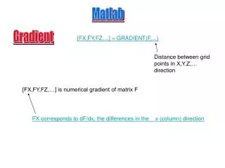
Matlab
Matlab. Gradient. [FX,FY,FZ,...] = GRADIENT(F,...). Distance between grid points in X,Y,Z,… direction. [FX,FY,FZ,…] is numerical gradient of matrix F. FX corresponds to dF/dx, the differences in the x (column) direction. y. (1,5). (2,5). (3,5). (4,5). (5,5). (1,4). (2,4). (3,4).

Matlab
E N D
Presentation Transcript
Matlab Gradient [FX,FY,FZ,...] = GRADIENT(F,...) Distance between grid points in X,Y,Z,… direction [FX,FY,FZ,…] is numerical gradient of matrix F FX corresponds to dF/dx, the differences in the x (column) direction
y (1,5) (2,5) (3,5) (4,5) (5,5) (1,4) (2,4) (3,4) (4,4) (5,4) (1,3) (2,3) (3,3) (4,3) (5,3) x (1,2) (2,2) (3,2) (4,2) (5,2) (1,1) (2,1) (3,1) (4,1) (5,1) Example [x,y] = meshgrid(-2:.2:2, -2:.2:2); z = x .* exp(-x.^2 - y.^2); [px,py] = gradient(z,.2,.2); contour(z),hold on, quiver(px,py), hold off [x,y] = meshgrid(-2:1:2, -2:1:2) Create a mesh on the domain of the function z. Examples: x(4,5)=1 y(4,5)=2 x(2,2)=-1 y(2,5)=2
y (1,5) (2,5) (3,5) (4,5) (5,5) (1,4) (2,4) (3,4) (4,4) (5,4) (1,3) (2,3) (3,3) (4,3) (5,3) x (1,2) (2,2) (3,2) (4,2) (5,2) (1,1) (2,1) (3,1) (4,1) (5,1) [x,y] = meshgrid(-2:.2:2, -2:.2:2); z = x .* exp(-x.^2 - y.^2); [px,py] = gradient(z,.2,.2); contour(z),hold on, quiver(px,py), hold off z=x.*exp(-x.^2-y.^2) Element by element operation X(4,5)=1 Y(4,5)=2 Z(4,5)=1*exp(-1^2-2^2)=exp(-5)=0.0067 -0.0007 -0.0067 0 0.0067 0.0007 -0.0135 -0.1353 0 0.1353 0.0135 -0.0366 -0.3679 0 0.3679 0.0366 -0.0135 -0.1353 0 0.1353 0.0135 -0.0007 -0.0067 0 0.0067 0.0007
y (1,5) (2,5) (3,5) (4,5) (5,5) (1,4) (2,4) (3,4) (4,4) (5,4) (1,3) (2,3) (3,3) (4,3) (5,3) x (1,2) (2,2) (3,2) (4,2) (5,2) (1,1) (2,1) (3,1) (4,1) (5,1) -0.0007 -0.0067 0 0.0067 0.0007 -0.0135 -0.1353 0 0.1353 0.0135 -0.0366 -0.3679 0 0.3679 0.0366 -0.0135 -0.1353 0 0.1353 0.0135 -0.0007 -0.0067 0 0.0067 0.0007 [x,y] = meshgrid(-2:.2:2, -2:.2:2); z = x .* exp(-x.^2 - y.^2); [px,py] = gradient(z,.2,.2); contour(z),hold on, quiver(px,py), hold off [px,py]=gradient(z,1,1) px = -0.0061 0.0003 0.0067 0.0003 -0.0061 -0.1219 0.0067 0.1353 0.0067 -0.1219 -0.3312 0.0183 0.3679 0.0183 -0.3312 -0.1219 0.0067 0.1353 0.0067 -0.1219 -0.0061 0.0003 0.0067 0.0003 -0.0061 py = -0.0128 -0.1286 0 0.1286 0.0128 -0.0180 -0.1806 0 0.1806 0.0180 0 0 0 0 0 0.0180 0.1806 0 -0.1806 -0.0180 0.0128 0.1286 0 -0.1286 -0.0128
CONTOUR(Z) is a contour plot of matrix Z treating the values in Z as heights above a plane. A contour plot are the level curves of Z for some values V. The values V are chosen automatically. [x,y] = meshgrid(-2:.2:2, -2:.2:2); z = x .* exp(-x.^2 - y.^2); [px,py] = gradient(z,.2,.2); contour(z),hold on, quiver(px,py), hold off px = -0.0061 0.0003 0.0067 0.0003 -0.0061 -0.1219 0.0067 0.1353 0.0067 -0.1219 -0.3312 0.0183 0.3679 0.0183 -0.3312 -0.1219 0.0067 0.1353 0.0067 -0.1219 -0.0061 0.0003 0.0067 0.0003 -0.0061 py = -0.0128 -0.1286 0 0.1286 0.0128 -0.0180 -0.1806 0 0.1806 0.0180 0 0 0 0 0 0.0180 0.1806 0 -0.1806 -0.0180 0.0128 0.1286 0 -0.1286 -0.0128 z = x .* exp(-x.^2 - y.^2);
[x,y] = meshgrid(-2:.2:2, -2:.2:2); z = x .* exp(-x.^2 - y.^2); [px,py] = gradient(z,.2,.2); contour(z),hold on, quiver(px,py), hold off HOLD ON holds the current plot and all axis properties so that subsequent graphing commands add to the existing graph. HOLD OFF returns to the default mode whereby PLOT commands erase the previous plots and reset all axis properties before drawing new plots.
Matlab Divergence: DIV = DIVERGENCE(X,Y,Z,U,V,W) computes the divergence of a 3-D vector field U,V,W. The arrays X,Y,Z define the coordinates for U,V,W and must be monotonic and 3-D plaid (as if produced by MESHGRID). Example: load wind div = divergence(x,y,z,u,v,w); slice(x,y,z,div,[90 134],[59],[0]); shading interp daspect([1 1 1]) camlight
load wind div = divergence(x,y,z,u,v,w); slice(x,y,z,div,[90 134],[59],[0]); shading interp daspect([1 1 1]) camlight Slice at (90,59,0) Wind is an array of (41,35,15). Origin: (70.2,17.5,0) End: (134.3, 60, 16) z y x
load wind div = divergence(x,y,z,u,v,w); slice(x,y,z,div,[90 134],[59],[0]); shading interp daspect([1 1 1]) camlight
load wind div = divergence(x,y,z,u,v,w); slice(x,y,z,div,[90 134],[59],[0]); shading interp daspect([1 1 1]) camlight
load wind div = divergence(x,y,z,u,v,w); slice(x,y,z,div,[90 134],[59],[0]); shading interp daspect([1 1 1]) camlight
Curl: [CURLX, CURLY, CURLZ, CAV] = CURL(X,Y,Z,U,V,W) computes the curl and angular velocity perpendicular to the flow (in radians per time unit) of a 3D vector field U,V,W. The arrays X,Y,Z define the coordinates for U,V,W and must be monotonic and 3D plaid (as if produced by MESHGRID). Ω Angular Velocity:
Example: load wind cav = curl(x,y,z,u,v,w); slice(x,y,z,cav,[90 134],[59],[0]); shading interp daspect([1 1 1]); axis tight colormap hot(16) camlight
Laplacien L = DEL2(U), when U is a matrix, is a discrete approximation of 0.25*del^2 u = (d^2u/dx^2 + d^2/dy^2)/4. The matrix L is the same size as U, with each element equal to the difference between an element of U and the average of its four neighbors.