Download
1 / 37
400 likes | 593 Views
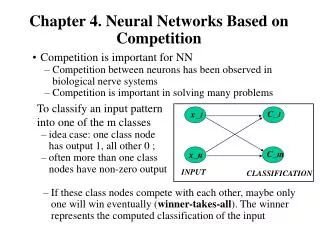
C_ 1. x_ 1. C_m. x_n. INPUT. CLASSIFICATION. Chapter 4. Neural Networks Based on Competition. To classify an input pattern into one of the m classes idea case: one class node has output 1, all other 0 ; often more than one class nodes have non-zero output.

E N D
C_1 x_1 C_m x_n INPUT CLASSIFICATION Chapter 4. Neural Networks Based on Competition • To classify an input pattern into one of the m classes • idea case: one class node has output 1, all other 0 ; • often more than one class nodes have non-zero output Competition is important for NN Competition between neurons has been observed in biological nerve systems Competition is important in solving many problems • If these class nodes compete with each other, maybe only one will win eventually (winner-takes-all). The winner represents the computed classification of the input
Winner-takes-all (WTA): • Among all competing nodes, only one will win and all others will lose • We mainly deal with single winner WTA, but multiple winners WTA are possible (and useful in some applications) • Easiest way to realize WTA: have an external, central arbitrator (a program) to decide the winner by comparing the current outputs of the competitors (break the tie arbitrarily) • This is biologically unsound (no such external arbitrator exists in biological nerve system).
y_j y_i y_j x_k y_i Ways to realize competition in NN Lateral inhibition (Maxnet, Mexican hat) output of each node feeds to others through inhibitory connections (with negative weights) Resource competition output of x_k is distributed to y_i and y_j proportional to w_ki and w_kj, as well as y_i and y_j self decay biologically sound • Learning methods in competitive networks • Competitive learning • Kohonen learning (self-organizing map, SOM) • Counter-propagation net • Adaptive resonance theory (ART) in Ch. 5
Fixed-weight Competitive Nets • Maxnet • Lateral inhibition between • competitors • Notes: • Competition: • iterative process until the net stabilizes (at most one node with positive activation) • where m is the # of competitors • too small: takes too long to converge • too big: may suppress the entire network (no winner)
Mexical Hat • Architecture: For a given node, • close neighbors: cooperative (mutually excitatory , w > 0) • farther away neighbors: competitive (mutually inhibitory,w < 0) • too far away neighbors: irrelevant (w = 0) • Need a definition of distance (neighborhood): • one dimensional: ordering by index (1,2,…n) • two dimensional: lattice
Equilibrium: • negative input = positive input for all nodes • winner has the highest activation; • its cooperative neighbors also have positive activation; • its competitive neighbors have negative activations.
Hamming Network • Hamming distance of two vectors, of dimension n, • Number of bits in disagreement. • In bipolar:
Suppose a space of patterns is divided into k classes, each class has an exampler (representative) vector . • An input belongs to class i, if and only if is closer to than to any other , i.e., • Hamming net is such a classifier: • Weights: let represent class j • The total input to
Upper layer: MAX net • it takes the y_in as its initial value, then iterates toward stable state • one output node with highest y_in will be the winner because its weight vector is closest to the input vector • As associative memory: • each corresponds to a stored pattern; • pattern connection/completion; • storage capacity total # of nodes: k total # of patterns stored: k capacity: k (or k/k = 1)
W_ij decay • Implicit lateral inhibition by competing limited resources: the activation of the input nodes y_1 y_j y_m x_i
Competitive Learning • Unsupervised learning • Goal: • Learn to form classes/clusters of examplers/sample patterns according to similarities of these exampers. • Patterns in a cluster would have similar features • No prior knowledge as what features are important for classification, and how many classes are there. • Architecture: • Output nodes: Y_1,…….Y_m, representing the m classes • They are competitors (WTA realized either by an external procedure or by lateral inhibition as in Maxnet)
Training: • Train the network such that the weight vector w.j associated with Y_j becomes the representative vector of the class of input patterns Y_j is to represent. • Two phase unsupervised learning • competing phase: • apply an input vector randomly chosen from sample set. • compute output for all y: • determine the winner (winner is not given in training samples so this is unsupervised) • rewarding phase: • the winner is reworded by updating its weights (weights associated with all other output nodes are not updated) • repeat the two phases many times (and gradually reduce the learning rate) until all weights are stabilized.
Weight update: • Method 1: Method 2 • In each method, is moved closer to x • Normalizing the weight vector to unit length after it is updated x-w_j x+w_j a(x-w_j) x x ax w_j w_j +a(x-w_j) w_j w_j+ ax
w_j(0) w_j(3) w_j(1) S(3) S(1) w_j(2) S(2) • is moving to the center of a cluster of sample vectors after repeated weight updates • Three examplers: • S(1), S(2) and S(3) • Initial weight vector w_j(0) • After successively trained • by S(1), S(2), and S(3), • the weight vector • changes to w_j(1), • w_j(2), and w_j(3)
Examples • A simple example of competitive learning (pp. 172-175) • 4 vectors of dimension 4 in 2 classes (4 input nodes, 2 output nodes) • S(1) = (1, 1, 0, 0) S(2) = (0, 0, 0, 1) • S(3) = (1, 0, 0, 0) S(4) = (0, 0, 1, 1) • Initialization: , weight matrix: • Training with S(1)
Similarly, after training with • S(2) = (0, 0, 0, 1) , • in which class 1 wins, • weight matrix becomes • At the end of the first iteration • (each of the 4 vectors are used), • weight matrix becomes • Reduce • Repeat training. After 10 • iterations, weight matrix becomes • S(1) and S(3) belong to class 2 • S(2) and S(4) belong to class 1 • w_1 and w_2 are the centroids of the two classes
Comments • Ideally, when learning stops, each is close to the centroid of a group/cluster of sample input vectors. • To stabilize , the learning rate may be reduced slowly toward zero during learning. • # of output nodes: • too few: several clusters may be combined into one class • too many: over classification • ART model (later) allows dynamic add/remove output nodes • Initial : • training samples known to be in distinct classes, provided such info is available • random (bad choices may cause anomaly)
w_2 w_1 Example will always win no matter the sample is from which class is stuck and will not participate in learning unstuck: let output nodes have some conscience temporarily shot off nodes which have had very high winning rate (hard to determine what rate should be considered as “very high”)
Kohonen Self-Organizing Maps (SOM) • Competitive learning (Kohonen 1982) is a special case of SOM (Kohonen 1989) • In competitive learning, • the network is trained to organize input vector space into subspaces/classes/clusters • each output node corresponds to one class • the output nodes are not ordered: random map cluster_1 • The topological order of the three clusters is 1, 2, 3 • The order of their maps at output nodes are 2, 3, 1 • The map does not preserve the topological order of the training vectors cluster_2 w_2 w_3 cluster_3 w_1
Topographic map • a mapping that preserves neighborhood relations between input vectors, (topology preserving or feature preserving). • if are two neighboring input vectors ( by some distance metrics), • their corresponding winning output nodes (classes), i and j must also be close to each other in some fashion • one dimensional: line or ring, node i has neighbors or • two dimensional:grid. rectangular: node(i, j) has neighbors: hexagonal: 6 neighbors
Biological motivation • Mapping two dimensional continuous inputs from sensory organ (eyes, ears, skin, etc) to two dimensional discrete outputs in the nerve system. • Retinotopic map: from eye (retina) to the visual cortex. • Tonotopic map: from the ear to the auditory cortex • These maps preserve topographic orders of input. • Biological evidence shows that the connections in these maps are not entirely “pre-programmed” or “pre-wired” at birth. Learning must occur after the birth to create the necessary connections for appropriate topographic mapping.
SOM Architecture • Two layer network: • Output layer: • Each node represents a class (of inputs) • Neighborhood relation is defined over these nodes Each node cooperates with all its neighbors within distance R and competes with all other output nodes. • Cooperation and competition of these nodes can be realized by Mexican Hat model R = 0: all nodes are competitors (no cooperative) random map R > 0: topology preserving map
SOM Learning • Initialize , and to a small value • For a randomly selected input sample/exampler determine the winning output node J either is maximum or is minimum • For all output node j with , update the weight • Periodically reduce and R slowly. • Repeat 2 - 4 until the network stabilized.
Notes • Initial weights: small random value from (-e, e) • Reduction of : Linear: Geometric: may be 1 or greater than 1 • Reduction of R: should be much slower than reduction. R can be a constant through out the learning. • Effect of learning For each input x, not only the weight vector of winner J is pulled closer to x, but also the weights of J’s close neighbors (within the radius of R). • Eventually, becomes close (similar) to . The classes they represent are also similar. • May need large initial R
Examples • A simple example of competitive learning (pp. 172-175) • 4 vectors of dimension 4 in 2 classes (4 input nodes, 2 output nodes) • S(1) = (1, 1, 0, 0) S(2) = (0, 0, 0, 1) • S(3) = (1, 0, 0, 0) S(4) = (0, 0, 1, 1) • Initialization: , weight matrix: • Training with S(1)
How to illustrate Kohonen map • Input vector: 2 dimensional Output vector: 1 dimensional line/ring or 2 dimensional grid. Weight vector is also 2 dimension • Represent the topology of output nodes by points on a 2 dimensional plane. Plotting each output node on the plane with its weight vector as its coordinates. • Connecting neighboring output nodes by a line output nodes: (1, 1) (2, 1) (1, 2) weight vectors: (0.5, 0.5) (0.7, 0.2) (0.9, 0.9) C(1, 2) C(1, 1) C(2, 1)
Traveling Salesman Problem (TSP) by SOM • Each city is represented as a 2 dimensional input vector (its coordinates (x, y)), • Output nodes C_j form a one dimensional SOM, each node corresponds to a city. • Initially, C_1, ... , C_n have random weight vectors • During learning, a winner C_j on an input (x, y) of city I, not only moves its w_j toward (x, y), but also that of of its neighbors (w_(j+1), w_(j-1)). • As the result, C_(j-1) and C_(j+1) will later be more likely to win with input vectors similar to (x, y), i.e, those cities closer to I • At the end, if a node j represents city I, it would end up to have its neighbors j+1 or j-1 to represent cities similar to city I (i,e., cities close to city I). • This can be viewed as a concurrent greedy algorithm
Initial position • Two candidate solutions: • ADFGHIJBC • ADFGHIJCB
Counter propagation network (CPN) • Basic idea of CPN • Purpose: fast and coarse approximation of vector mapping • not to map any given x to its with given precision, • input vectors x are divided into clusters/classes. • each cluster of x has one output y, which is (hopefully) the average of for all x in that class. • Architecture: Simple case: FORWARD ONLY CPN, from class to (output) features from (input) features to class
Learning in two phases: • training sample x:y where is the precise mapping • Phase1: is trained by competitive learning to become the representative vector of a cluster of input vectors x (use sample x only) 1. For a chosen x, feedforward to determined the winning 2. 3. Reduce , then repeat steps 1 and 2 until stop condition is met • Phase 2: is trained by delta rule to be an average output of where x is an input vector that causes to win (use both x and y). 1. For a chosen x, feedforward to determined the winning 2. (optional) 3. 4. Repeat steps 1 – 3 until stop condition is met
Notes • A combination of both unsupervised learning (for in phase 1) and supervised learning (for in phase 2). • After phase 1, clusters are formed among sample input x , each is a representative of a cluster (average). • After phase 2, each cluster j maps to an output vector y, which is the average of • View phase 2 learning as following delta rule
After training, the network works like a look-up of math table. • For any input x, find a region where x falls (represented by the wining z node); • use the region as the index to look-up the table for the function value. • CPN works in multi-dimensional input space • More cluster nodes (z), more accurate mapping.
Full CPN • If both we can establish bi-directional approximation • Two pairs of weights matrices: V ( ) and U ( ) for approx. map x to W ( ) and T ( ) for approx. map y to • When x:y is applied ( ), they can jointly determine the winner J or separately for • pp. 196 –206 for more details