Chapter 5 Estimating Demand Functions
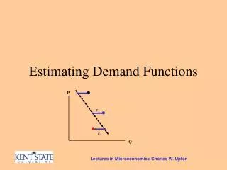
Chapter 5 Estimating Demand Functions. Identification Problem. The inability to distinguish between moves along a demand curve and shifts in supply and/or demand that reflect changes in behavior. S 99. D 99. S 98. D 98. Estimated Demand Contrasted with Actual Demand. D. Price. S 97.


Chapter 5 Estimating Demand Functions
E N D
Presentation Transcript
Identification Problem The inability to distinguish between moves along a demand curve and shifts in supply and/or demand that reflect changes in behavior
S99 D99 S98 D98 Estimated Demand Contrasted with Actual Demand D Price S97 D| D97 Quantity
Alternative Methods of Estimating Demand • Consumer interviews. • Market experiments. • Regression analysis.
Regression Analysis • A statistical technique that describes the way in which one variable is related to another • Used to estimate demand • Assumes that the mean value of the dependent variable is a linear function of the independent variable Yi = A + BXi + ei
The Mean Value of X Falls on the Population Regression Line Price . A + BX Population regression line . Y2 e2 = 1.5 . . e1 = -1 A + BX2 Y1 A + BX1 X1 X2 Quantity
Ŷ = a + bxt Ŷ = the value of the dependent variable predicted by the regression line a = the y-intercept of the regression line b = the slope of the regression line Xt = the value of the independent variable at t
n i = 1 (Yi - a - bxi)2 n i = 1 Method of Least Squares (Yi - Ŷi)2 =
y y x x Coefficient of Determination • Commonly called the “R-squared” • measures goodness of fit of the estimated regression line • varies between 0 and 1
Multiple Regression Includes two or more independent variables Yi = A + b1Xi + b2Pi + ei where: Yi = sales xi = selling expense Pi = price
Regression Analysis • Given data on relevant variables, the empirical method of Regression Analysis can be used to estimate demand functions. We will begin by considering a simplified version of a demand function showing quantity demanded as a function of only price. Such a demand function would clearly be inadequate to successfully estimate a demand function. We use this simplified example of a demand function merely as a means of illustrating the technique of regression analysis. Once the technique is fully developed, we will proceed to estimate more realistic demand functions.
Quantity Demanded and Price • Let Yt be quantity demanded (i.e. Sales) in period t. • Let Xt be the price charged in period t. Plotting a firm’s historical data for these two variables we may have the graph shown on the right. • As the graph reveals, there is apparently a negative relationship between Sales and Price, i.e. as Price increases, Sales also tends to decrease.
Fitting A Line To Data • The relationship between Ytand Xt can be represented (albeit imperfectly) by a line that “best fits” the scatter of points. The line shown is defined by its intercept, a, and its slope, b. Notice, however, that the actual points do not fall exactly on the line. This is due to the fact that Sales may be partly determined by price, but other factors such as advertising, which are not taken into account, also affect Sales.
Fitting A Line To Data (continued) • Regression analysis is basically focused on methods of estimating lines that best fit data, such as the one shown in the previous slide. • Each dot shown in the graph can be broken up in to two pieces: the amount of Sales, , predicted by the line, and the resulting error (or “residual”) in prediction, et. Or, mathematically, • Or, since: • We have:
Method of Ordinary Least-Squares • Our goal is thus to estimate a line by finding a value for a and b such that resulting line “best fits” the data. We do so by finding values of a and b such that the sum of squared errors is minimized. That is, we can write the sum of squared errors as: • where n is the number of observations in our sample of data. This sum of squared errors can be minimized using differential calculus. Leaving out the details, minimizing this equation with respect to a and b yields the following results: • and
Interpreting The OLS Output • R Square: A measure of the “goodness of fit.” It is the proportion of the variation in the dependent variable explained by the regression. It has a maxmimum of 1 (100%) meaning an perfect fit, and a minimum of 0 (0%), meaning no fit at all. Thus, the closer to 1, the better the fit. • Standard Error: The size of the typical error (et). • Significance FThis shows the probability of obtaining the estimated values of the X coefficients from a sample regression if it were true that all the population's X coefficients are simultaneously equal to zero. If the Significance F is less than our chosen level of significance, then we can conclude that the model as a whole is statistically significant in explaining the values of the dependent variable
Interpreting The OLS Output • Coefficients: The estimated value for a and b for our model. The “Intercept” is the estimate for a. The coefficient for “Price” is our estimate for b. • P-Value: Used in hypothesis testing to test whether a sample estimate of a coefficient is statistically different from zero. It represents the probability of achieving the estimated coefficient for the sample at hand, if in fact the population's coefficient were zero. If the p-value is less than the chosen level of significance, then the zero hypothesis is rejected.
Forecasting Using Regression Output • Given an estimated regression, we can use it to forecast or make predictions. For example, suppose we have our estimated equation: • If we decide to seta price of $4 next period, we can predict sales as:
Forecasting Using Regression Output (Continued) • Interval estimates: The previous forecast was a “point estimate” (i.e. an estimated number). As an alternative, we can estimate an interval that we are reasonably sure will contain the actual value of sales given advertising is $425. To do so we take our point estimate and add and subtract 2 times the standard error, thus creating an approximate 95% confidence interval*: • Or, in this case, • Or, the 95% confidence interval is approximately: (2360.38, 7609.16). • [*It should be noted that this interval estimate is only reliable if the independent variable’s value (i.e. the value chosen for Price) is close to its mean value. Values not close to their mean require a more complicated formula.]
Multiple Regression Analysis • We may consider models with multiple independent variables. That is, we can consider advertising along with price, income, price of related goods, etc. Our regression model becomes: • Salest = a + b1Pricet + b2Advertisingt + b3Incomet + b4PRGt + et • Given data on the 4 independent variables, we can estimate values for a and b1 through b4 using the method of ordinary least-squares. Doing so by-hand is difficult, but computer programs such as Excel can estimate such regressions quite easily.
Predicted Equation • Using the coefficients from our regression, we have the following predicted equation: • Given values for the independent variables, we can predict values for Sales. We can also consider the statistical importance of the independent variables as we did earlier.
Goodness of Fit in Multiple Regression Models • Notice that the R Square increased from about 0.615 for our model with only Price, to about 0.863 for our model that adds Advertising, Income and PRG. Note, however, that to compare two regressions with the same dependent variable (Sales) but differing numbers of independent variables, we must use the Adjusted R Square to determine which model is performing better. Thus, the model with just Price has an Adjusted R Square of 0.587, whereas our multiple regression model has an Adjusted R Square of 0.813. Thus our multiple regression model indeed seems to be outperforming our model with just Price as an independent variable.
Estimating Elasticities • Elasticities at the “means” • Mean values: • Price= 3.11 • Advertising=141.44 • Income=180.53 • PRG=3.4 • predicted sales = 7630.65
Estimating Elasticities (continued) • Price: • Advertising: • Income: • PRG (cross):
Estimating Elasticities (continued) • Constant Elasticities: Log Transformations: • Regressing the natural log of the dependent variable (sales) on the natural logs of the independent variables produces coefficients that are estimates of constant elasticities.
Standard error of estimate • A measure of the amount of scatter of individual observations about the regression line • Useful for constructing prediction intervals • Y-hat +/- 2 standard errors
F-statistic • Tells us whether or not the group of independent variables explains a statistically significant portion of the variation in the dependent variable. • Large values of the F-statistic indicate that at least one of the independent variables is helping to explain variation in the dependent variable.
t-statistic • Tells us whether or not each particular independent variable explains a statistically significant portion of the variation in the dependent variable • All else equal, larger values for the t-stat are better • Rule of Thumb: as long as the t-stat is greater than 2, the independent variable belongs in the equation
Multicollinearity • A situation in which two or more of the independent variables are highly correlated • Indicated by high r-squared and significant F-stat, but low t-stats for the independent variables
Serial Correlation • A situation in which error terms are not independent of one another over time • To detect, consider the Durbin-Watson statistic • Rule of Thumb: If the DW is close to 2, serial correlation is not present. If the DW is close to 1 or 4, serial correlation is present
Further Analysis of Residuals • Plot scatters of the residuals against each independent variable • There are problems with the regression analysis if patterns emerge