Download
1 / 94
940 likes | 1.13k Views
Q 4 – 1 a. Let T = number of TV advertisements R = number of radio advertisements N = number of newspaper advertisements. Q 4 – 1 a. cont’d. Optimal Solution: T = 4, R = 14, N = 10 Allocation: TV 2,000(4) = $8000 Radio 300(14) = $4,200

E N D
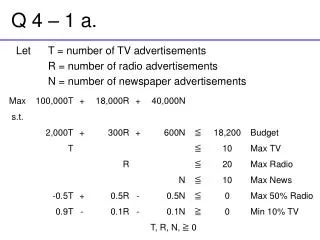
Q 4 – 1 a. Let T = number of TV advertisements R = number of radio advertisements N = number of newspaper advertisements
Q 4 – 1 a. cont’d Optimal Solution: T = 4, R = 14, N = 10 Allocation: TV 2,000(4) = $8000 Radio 300(14) = $4,200 News 600(10) = $6,000 Objective Function Value (Expected number of audience): 100,000(4) + 18,000(14) + 40,000(10) =1,052,000
Q 4 – 1 b. cont’d The dual price for the budget constraint is 51.30. Thus, a $100 increase in budget should provide an increase in audience coverage of approximately 5,130. The RHS range for the budget constraint will show this interpretation is correct.
Q 4 – 10 a. Let S = the proportion of funds invested in stocks B = the proportion of funds invested in bonds M = the proportion of funds invested in mutual funds C = the proportion of funds invested in cash
Q 4 – 10 a. cont’d From computer results, the optimal allocation among the four investment alternatives is Stocks 40.0% Bonds 14.5% Mutual Funds 14.5% Cash 30.0% The annual return associated with the optimal portfolio is 5.4% The total risk = 0.409(0.8) + 0.145(0.2) + 0.145(0.3) + 0.300(0.0) = 0.4
Q 4 – 10 b. Changing the RHS value for constraint 2 to 0.18 and resolving using computer, we obtain the following optimal solution: Stocks 0.0% Bonds 36.0% Mutual Funds 36.0% Cash 28.0% The annual return associated with the optimal portfolio is 2.52% The total risk = 0.0(0.8) + 0.36(0.2) + 0.36(0.3) + 0.28(0.0) = 0.18
Q 4 – 10 c. Changing the RHS value for constraint 2 to 0.7 and resolving using computer, we obtain the following optimal solution: Stocks 75.0% Bonds 0.0% Mutual Funds 15.0% Cash 10.0% The annual return associated with the optimal portfolio is 8.2% The total risk = 0.75(0.8) + 0.0(0.2) + 0.15(0.3) + 0.10(0.0) = 0.65
Q 4 – 10 d. Note that a maximum risk of 0.7 was specified for this aggressive investor, but that the risk index for the portfolio is only 0.67. Thus, this investor is willing to take more risk than the solution shown above provides. There are only two ways the investor can become even more aggressive: increase the proportion invested in stocks to more than 75% or reduce the cash requirement of at least 10% so that additional cash could be put into stocks. For the data given here, the investor should ask the investment advisor to relax either or both of these constraints.
Q 4 – 10 e. Defining the decision variables as proportions means the investment advisor can use the linear programming model for any investor, regardless of the amount of the investment. All the investor advisor needs to do is to establish the maximum total risk for the investor and resolve the problem using the new value for maximum total risk.
A – 2 (a) Let S = Tablespoons of Strawberry C = Tablespoons of Cream V = Tablespoons of Vitamin A = Tablespoons of Artificial sweetener T = Tablespoons of Thickening agent
A – 2 (c) Since u1*, u5*, u6* > 0, the 1st, 5th, and 6th constraints are binding.
Data Envelopment Analysis The Langley County School District is trying to determine the relative efficiency of its three high schools. In particular, it wants to evaluate Roosevelt High. The district is evaluating performances on SAT scores, the number of seniors finishing high school, and the number of students who enter college as a function of the number of teachers teaching senior classes, the prorated budget for senior instruction, and the number of students in the senior class.
Input RooseveltLincolnWashington Senior Faculty 37 25 23 Budget ($100,000's) 6.4 5.0 4.7 Senior Enrollments 850 700 600
Output RooseveltLincoln Washington Average SAT Score 800 830 900 High School Graduates 450 500 400 College Admissions 140 250 370
Data Envelopment Analysis • Decision Variables E = Fraction of Roosevelt's input resources required by the composite high school w1 = Weight applied to Roosevelt's input/output resources by the composite high school w2 = Weight applied to Lincoln’s input/output resources by the composite high school w3 = Weight applied to Washington's input/output resources by the composite high school
Data Envelopment Analysis • Objective Function Minimize the fraction of Roosevelt High School's input resources required by the composite high school: MIN E
Data Envelopment Analysis • Constraints Sum of the Weights is 1: (1) w1 + w2 + w3 = 1 Output Constraints: Since w1 = 1 is possible, each output of the composite school must be at least as great as that of Roosevelt: (2) 800w1 + 830w2 + 900w3> 800 (SAT Scores) (3) 450w1 + 500w2 + 400w3> 450 (Graduates) (4) 140w1 + 250w2 + 370w3> 140 (College Admissions)
Input Constraints: The input resources available to the composite school is a fractional multiple, E, of the resources available to Roosevelt. Since the composite high school cannot use more input than that available to it, the input constraints are: (5) 37w1 + 25w2 + 23w3< 37E (Faculty) (6) 6.4w1 + 5.0w2 + 4.7w3< 6.4E (Budget) (7) 850w1 + 700w2 + 600w3< 850E (Seniors) Non-negativity of variables: E, w1, w2, w3> 0
Data Envelopment Analysis OBJECTIVE FUNCTION VALUE = 0.765 VARIABLEVALUE E 0.765 W1 0.000 W2 0.500 W3 0.500
Conclusion The output shows that the composite school is made up of equal weights of Lincoln and Washington. Roosevelt is 76.5% efficient compared to this composite school when measured by college admissions (because of the 0 slack on this constraint (#4)). It is less than 76.5% efficient when using measures of SAT scores and high school graduates (there is positive slack in constraints 2 and 3.)
Data Envelopment Analysis • (1) Relative Comparison • (2) Multiple Inputs and Outputs • (3) Efficiency Measurement (0%-100%) • (4) Avoid the Specification Error between Inputs and Outputs • (5) Production/Cost Analysis
Case : 1 input – 1 output Table 1.1 : 1 input – 1 output Case
Efficiency Frontier E G Output F C A H B D 0 Employees Figure 1.1:Comparison of efficiencies in 1 input–1 output case
Efficiency Frontier E G Output F C A Regression Line H B D 0 Employees Figure 1.2 : Regression Line and Efficiency Frontier
Table 1.2 : Efficiency 1 = C > G > A> B > E > D = F > H = 0.4
Efficiency Frontier Output C D2 D1 D 0 Employee Figure 1.3 : Improvement of Company D
Case : 2 inputs – 1 output Table 1.3 : 2 inputs – 1 output Case
Production Possibility Set G F C A I Offices/Sales E D B Efficiency Frontier H 0 Employees/Sales Figure 1.4 : 2 inputs – 1 output Case
C A Offices/Sales A1 A2 B 0 Employees/Sales Figure 1.5 : Improvement of Company A
Case : 1 input – 2 outputs Table 1.4 : 1 input – 2 outputs Case
A1 B C A Efficiency Frontier D F Sales/Office Production Possibility Set E1 G E 0 Customers/Office Figure 1.6 : 1 input – 2 outputs Case
Case : Multiple inputs – Multiple outputs Table 1.5 : Example of Multiple inputs–Multiple outputs Case
Example Problem Table 1.6 : 2 inputs – 1 output Case
Efficiency Frontier E A D A1 F C 0 Figure 1.7 : Efficiency of DMU A