The Normal Distribution
The Normal Distribution . Lesson 1. Objectives. To introduce the normal distribution The standard normal distribution Finding probabilities under the curve. Normal Distributions. Normal distributions are used to model continuous variables in many different situations.

The Normal Distribution
E N D
Presentation Transcript
The Normal Distribution Lesson 1
Objectives • To introduce the normal distribution • The standard normal distribution • Finding probabilities under the curve
Normal Distributions Normal distributions are used to model continuous variables in many different situations. For example, a normal distribution could be used to model the height of students. We can transform our normal distribution into a standardnormal distribution…
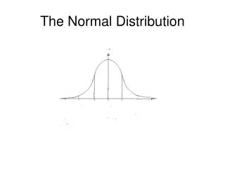
The standard normal variable The standard normal variable is usually denoted by Z It has a mean =0 and a standard deviation of =1 ) The curve fits within ±4 standard deviations from the mean The curve is designed so that the total area underneath the curve is 1
Find P (Z≤a) To do this we begin with a sketch of the normal distribution
P (Z≤a) To do this we begin with a sketch of the normal distribution. We then mark a line to represent Z=a a
P (Z≤a) To do this we begin with a sketch of the normal distribution. We then mark a line to represent Z=a P(Z≤a) is the area under the curve to the left of a. For continuous distributions there is no difference between P(Z≤a) and P(Z<a) a
Ex1 Find P (Z<1.55) To do this we begin with a sketch of the normal distribution
Ex 1 Find P (Z<1.55) To do this we begin with a sketch of the normal distribution. We then mark a line to represent Z=1.55 a
Ex 1 Find P (Z<1.55) To do this we begin with a sketch of the normal distribution. We then mark a line to represent Z=a P(Z<1.55) is the area under the curve to the left of a. We now use the table to look up this probability a
The Normal Distribution Table • The table describes the positive half of the bell shaped curve… • (Z) is sometimes used as shorthand for P(Z<z)
Ex 1 Find P (Z<1.55) To do this we begin with a sketch of the normal distribution. We then mark a line to represent Z=a P(Z<1.55) is the area under the curve to the left of a. We now use the table to look up this probability P(Z<1.55) = 0.9394 a
Ex 2 Find P(Z>1.74) Note this result.. P(Z>a) = 1-P(Z<a) So P(Z>1.74) = 1 – P(Z<1.74) = 1 – (0.9591) = 0.0409
Ex 3 P(Z<-0.83) As our table only has values for the positive side of the distribution we must use symmetry…
Ex 3 P(Z<-0.83) We have reflected the curve in the vertical axis. P(Z<-0.83) = 1- P(0.83) = 1 – (0.7967) = 0.2033 This is a really useful technique P(Z<-a) = P(Z>a) = 1- P(Z<a)
This is a really useful result P(Z<-a) = 1 - P(Z<a)
Ex 4 P(-1.24<Z<2.16) P(Z<2.16) = 0.9846
Ex 4 P(-1.24<Z<2.16) P(Z<2.16) = 0.9846 P(Z<-1.24) = 1-P(Z<1.24) = 1-0.8925 = 0.1075
Ex 4 P(-1.24<Z<2.16) P(Z<2.16) = 0.9846 P(Z<-1.24) = 1-P(Z<1.24) = 1-0.8925 = 0.1075 P(-1.24<Z<2.16) = 0.9846 – 0.1075 = 0.8771
Recommended work… • Read through pages 177 and 178. • Do Exercise 9A p179

