Download

1 / 59
590 likes | 611 Views
The Quadrupole Cusp: A Universal Accelerator, or From Radiation Belts to Cosmic Rays. Robert Sheldon NSSTC Seminar, March 19, 2004. Outline. Quadrupoles Plasma Thermodynamics Acceleration Mechanisms and Entropy shocks, waves, reconnection and dipole

E N D
The Quadrupole Cusp: A Universal Accelerator, orFrom Radiation Belts to Cosmic Rays Robert Sheldon NSSTC Seminar, March 19, 2004
Outline • Quadrupoles • Plasma Thermodynamics • Acceleration Mechanisms and Entropy • shocks, waves, reconnection and dipole • Why a trap improves acceleration efficiency • How a Quadrupole Traps & Accelerates • Signatures of Quadrupole Acceleration • Application 1: Outer Radiation Belt Electrons • Application 2: Galactic Cosmic Rays
Introduction • Why is studying acceleration mechanisms important? • Fundamental physics (e.g. Nobel Prizes) • Usefulness in medicine, science, technology • Radiation therapy, advanced light sources, microwave ovens etc. • Prediction of harmful radiation to satellites and humans in space. • NASA goals, even Moon missions! • Plain fun.
Two “unsolved” physics problems • Source of the highly variable, outer radiation belt electrons • Source of Galactic cosmic rays.
Plasma Thermodynamics • A neglected field—so this discussion is very qualitative. (Please give me references!) • In ideal gases the Maxwell equilibrium is extremely well maintained by collisions • In plasmas, turbulence takes the place of collisions. But the long-range Coulomb interaction means that equilibrium is often attained very slowly. • Therefore one must get accustomed to non-Maxwellian distributions, and non-standard measures of temperature and entropy. E.g. kappas
What is Acceleration? • Entropy is often defined as S = Q/T. Thus highly energetic particles have low entropy. Often they are “bump-on-a-tail” distributions, or “power law” greater than Maxwellian. Such low-entropy conditions cannot happen spontaneously, so some other process must increase in entropy. Separating the two mechanisms, we have a classic heat-engine. Note: the entropy INCREASE of heat flow into the cold reservoir, is counterbalanced by the DECREASE of entropy into the Work.
Efficiency of Acceleration • The efficiency of a heat engine is easy to describe: e=W/Q1. The work produced for some amount of heat. We can also use a slightly modified definition by dividing by temperature, T: e=Sw/SQ • We can now use these definitions to categorize the various acceleration mechanisms that have been proposed for radiation belts and cosmic rays. • Waves Very Low < 10-4 • Reconnection Low < 10-3 • Fermi I and II Medium < 10-1 • Shocks Low < 10-3
Why does a Trap help? • Single-stage acceleration mechanisms operate very far from equilibrium. They therefore have a huge difference in entropy between W and Q, and are therefore inherently inefficient. Likewise environmental conditions are far from equilibrium, and are thus inherently unlikely. The product of these two situations = low density of accelerated particles. Energy Source * Efficiency * Probability = Power • A trap allows small impulses to be cumulative. The pulses are close to equilibrium and are also likely. Thus a trap = higher density of accelerated particles.
The Fermi-Trap Accelerator Waves convecting with the solar wind, compress trapped ions between the local |B| enhancement and the planetary bow shock, resulting in 1-D compression, or E// enhancement.
The Dipole Trap • The dipole trap has a positive B-gradient that causes particles to trap, by B-drift in the equatorial plane. There are 3 symmetries to the Dipole each of which has its own “constant of the motion” (Hamiltonian is periodic). 1)Gyromotion around B-field Magnetic moment, “”; 2) Reflection symmetry about equator Bounce invariant “J”; 3) Cylindrical symmetry about z-axis Drift invariant “L”
The Quadrupole Trap • A quadrupole is simply the sum of two dipoles. • Dipole moving through a magnetized plasma, heliosphere, magnetosphere, galactosphere • A binary system of magnetized objects –binary stars • A distributed current system-Earth’s core, supernovae • Quadrupoles have “null-points” which stably trap charged particles (eg. Paul trap used in atomic physics) • Maxwell showed that a perfect conducting plane would “reflect” a dipole & form a quadrupole
Why is the Dipole a better trap than Accelerator? • Three “adiabatic invariants” (, J, L) w/characteristic times of 1ms, 1s, 1000s • KAM theorem: the 3 adiabatic invariants are separated by factors of 1000 in time, and therefore do not “mix”. So dynamical evolution, or diffusive/stochastic “acceleration” is not fast. • Arnol’d diffusion, or chaotic motion in the Poincaré section, can lead to rapid diffusion if these “basins” are connected to each other--“Arnol’d web”
Kolmogorov, Arnol’d, Moser Theorem Earth orbit as Perturbed by Jupiter. Poincaré slice x vs. vX taken along the E-J line. Earth orbit if Jupiter were 50k Earth masses.
Rim fed, center exit Exit blocked by magnet Compressions mostly affect the low-energy part High-E particles are better trapped than Low-E Adiabatic invariant times separated by factor ~1000 Scattering (diffusion) out of the trap is difficult and de-energizing / deaccelerating. Center fed, rim exit Exit accessible Compressions affect whole distribution High-E particles less trapped than Low-E Adiabatic invariant times separated by factor ~10 Scattering out of trap is easy and may also energize/ accelerate Comparison of Dipole & Quadrupole
Quadrupole Trap in the Laboratory(Two 1-T magnets, -400V, 50mTorr)
Poincaré Plots? • Now that we know there are trapping regions of the cusp, e.g. periodic orbits, we can display those orbits with a Poincaré section. Then we can potentially demonstrate the invariant tori and chaotic orbits. • Unfortunately, I only realized the advantage of this approach after plotting 4000 trajectories T<drift-time and visually classifying them as “untrapped”, “trapped periodic”, and “trapped chaotic”. (Using 4 CPU weeks on dual AMD 1.8GHz) • So the Poincaré plot (many drift orbits) will have to wait for CPU time.
How does the Quadrupole Accelerate? • Mathematically, we say that the basins of chaos are interconnected, not constrained by invariant tori. They are connected in an Arnol’d web that allows rapid stochastic acceleration. • More prosaically, compressions adiabatically increase the particle energy, while the center of the trap acts as a “mixmaster” for redistributing that energy into other invariants. Consequently particles diffuse in energy very rapidly. • A comparison to Fermi I,II is highly instructive for understanding the mechanism.
Acceleration via Random Impulses • Fermi-I acceleration can be thought of as a 1-D compression of a magnetized plasma. It heats only in the E// direction. Eventually the pitchangle gets too small to be reflected by the upstream waves, and it escapes. If pitchangle diffusion occurs, a particle may convert E//E_perp, and continue to gain energy. • The waves, or compressive impulses need not be coherent or particularly large, especially if scattering is occurring. Thus the entropy of the energy source is relatively high, the probability is high = high efficiency acceleration. Observations support this.
Cusp OrientationWhen the cusp points toward the sun, it “opens”, when it points away, it “closes”. Likewise, SW pressure pulses will shrink the cusp as a whole, e.g. radially compressing it.
1-D compression, E// Upstream Alfven waves impinging on barrier Scattering inside trap due to waves Max Energy due to scale size of barrier (curvature) becoming ~ gyroradius Acceleration time exponentially increasing Critically depends on angle of SW B-field with shock 2-D compression, E_perp Compressional waves impinging on cusp Scattering inside trap due to quadrupole null point Max energy due to gyroradius larger than cusp radius (rigidity). Acceleration time exponentially increasing Critically depends on cusp angle with SW Fermi I,II vs Alfven I,II
Signatures of Cusp Acceleration • Gyroradius effects: r = (mE)1/2/qB. For a given topology, lighter masses will have higher cutoff energies. • Energy increase is exponentially increasing function of time. (like Fermi) • Scale size effects: the larger the cusp, and the larger B-field, the higher the cutoff E. • Output spectra have power law tails (not bump-on-tail nor exponential maxwellians.) • Given continuous input, output is also continuous.
Prediction Problems • The hazards of MeV electrons are greatest in the outer radiation belts (L~3-5), though they still exist for LEO orbits and the South Atlantic Anomaly. • MeV electrons penetrate, causing deep dielectric discharges, such as the Telstar 401 satellite loss. • The Geosynchronous orbit uniquely lies on the edge of a steep spatial and spectral gradient. Thus GEO poses a wildly variable MeV electron environment, which is nearly impossible to predict, both in principle and in practice. • Yet of all orbits, this is THE most crowded spot.
Details of Injection (#1&5) • They have a 24-48 hour typical rise time from a SW disturbance (shock, Dst storm, etc.) But can be as short as 8 hr (Jan 97) or as long as 72 hours. • The intensity roughly follows a solar cycle dependence but can vary by 3 orders of magnitude • The spectral hardness generally increases during the storm, but exhibits a “knee” that whose cutoff strongly depends on the unpredictable magnitude • Best correlation with Vsw (70%) but Bz or n_sw ruins it. Neither mechanical nor electrical SW driver
The Prediction Paradox • The storms we want to predict, are the BIG ones, but our best statistics are the little storms. Statistical precursors, neural nets, linear filters ALWAYS do better on the little storms, not the killer storms. • We will never achieve reasonable prediction until we understand how/where/why BIG storms occur. Everything else is gambling. • But the statistics have not led to better physics. Why is Vsw the best correlator? Especially since Dst is better correlated to Ey and AE to Bz. Why is Kp the best correlated ground-based index?
The Argument 1) Electrons, not protons are injected. 2) Radial gradients point to an external source that is NOT the solarwind, NOR the dipole trapped belts. 3) Risetimes are too slow (2 days) to be 1st order acceleration, more likely 2nd order stochastic, ordered by energy dependent exponential risetimes. 4) Neither AE nor Dst correlate as well as Kp. Global disturbances work better than tail or RC. 5) MLT enhancements begin at noon. 6) Low altitude data are consistent with simultaneous inward radial transport & PA scattering
Problems with Cusp Acceleration • We said that Cusp acceleration was continuous, given continuous injection. How then do we explain the abrupt injections observed in storms & McIlwain’s data? • The solution is topology. Abrupt changes in topology of the cusp also cause abrupt changes in output. The key is that the cusp is a POSITIVE feedback amplifier, and can be driven to the rails by appropriate input. • The plasma trapped in the cusp also contributes to the magnetic field topologymaking it stronger!
Model Predictions • MeV electrons are born in CDCs • Not solar wind Vsw but DVsw drives MeV e • Conditions amenable to driving plasma in the cusp are the predictors for MeV e events: • Cusp tilted toward the Sun. Solstices over equinox. • High momentum solar wind. • Bz northward during impact. Turbulence afterward. • The longer the CDC lasts, the higher the “knee”, and the harder the spectrum • MeV-Dst correlations are also due to DVsw
Scaling Laws • Brad ~ Bsurface= B0 • Bcusp ~ B0/Rstag3 • Erad= 5 MeV for Earth • Ecusp ~ v2perp~ (Bcuspr)2 ~ [(B0/Rstag3)Rstag] • m = E/B is constant Erad-planet~(Rstag-Earth/Rstag-planet)(B0-planet/B0-Earth)2Erad-Earth
Scaled Radiation Belts Planet Mercury Earth Mars Jupiter Saturn Uranus Neptune R STAG 1.4 10.4 1.25 65 20 20 25 B0 (nT) 330 31,000 < 6 430,000 21,000 23,000 14,000 ERAD 4 keV 5 MeV < 1.5 eV 150 MeV 1.2 MeV 1.4 MeV 0.42 MeV
More Predictions • The unpredictability arises from a strong non-linearity in the trapping ability of the cusp. Small misalignment of cusp & no CDC is formed. • Note that high Vsw usually means high DVsw, and simultaneously, higher seed energies for 2nd order Fermi acceleration. Thus a synergistic correlation. • Magnetic clouds are also geoeffective, but with very different properties than high speed streams (Jan 97) • CDC probably “evaporate” releasing lowest energy last, causing Time-Energy Dispersions. • Positive feedback means many inputs=same output