Download

1 / 35
350 likes | 538 Views
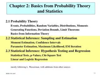
Chapter 2: Basics from Probability Theory and Statistics. 2.1 Probability Theory Events, Probabilities, Random Variables, Distributions, Moments Generating Functions, Deviation Bounds, Limit Theorems Basics from Information Theory 2.2 Statistical Inference: Sampling and Estimation

E N D
Chapter 2: Basics from Probability Theoryand Statistics • 2.1 Probability Theory • Events, Probabilities, Random Variables, Distributions, Moments • Generating Functions, Deviation Bounds, Limit Theorems • Basics from Information Theory • 2.2 Statistical Inference: Sampling and Estimation • Moment Estimation, Confidence Intervals • Parameter Estimation, Maximum Likelihood, EM Iteration • 2.3 Statistical Inference: Hypothesis Testing and Regression • Statistical Tests, p-Values, Chi-Square Test • Linear and Logistic Regression mostly following L. Wasserman, with additions from other sources
2.2 Statistical Inference: Sampling and Estimation A statistical model is a set of distributions (or regression functions), e.g., all unimodal, smooth distributions. A parametric model is a set that is completely described by a finite number of parameters, (e.g., the family of Normal distributions). Statistical inference: given a sample X1, ..., Xn how do we infer the distribution or its parameters within a given model. For multivariate models with one specific „outcome (response)“ variable Y, this is called prediction or regression, for discrete outcome variable also classification. r(x) = E[Y | X=x] is called the regression function.
Statistical Estimators A point estimator for a parameter of a prob. distribution is a random variable X derived from a random sample X1, ..., Xn. Examples: Sample mean: Sample variance: An estimator T for parameter is unbiased if ; otherwise the estimator has bias . An estimator on a sample of size n is consistent if Sample mean and sample variance are unbiased, consistent estimators with minimal variance.
Estimator Error Let = T() be an estimator for parameter over sample X1, ..., Xn. The distribution of is called the sampling distribution. The standard error for is: The mean squared error (MSE) for is: If bias 0 and se 0 then the estimator is consistent. The estimator is asymptotically Normal if converges in distribution to standard Normal N(0,1)
Nonparametric Estimation The empirical distribution function is the cdf that puts prob. mass 1/n at each data point Xi: A statistical functional T(F) is any function of F, e.g., mean, variance, skewness, median, quantiles, correlation The plug-in estimator of = T(F) is: Instead of the full empirical distribution, often compact data synopses may be used, such as histograms where X1, ..., Xn are grouped into m cells (buckets) c1, ..., cm with bucket boundaries lb(ci) and ub(ci) s.t. lb(c1) = , ub(cm) = , ub(ci) = lb(ci+1) for 1i<m, and freq(ci) = Histograms provide a (discontinuous) density estimator.
Parametric Inference: Method of Moments Compute sample moments: for j-th moment j Estimate parameter by method-of-moments estimator s.t. and and and ... (for some number of moments) Method-of-moments estimators are usually consistent and asympotically Normal, but may be biased
Parametric Inference:Maximum Likelihood Estimators (MLE) Estimate parameter of a postulated distribution f(,x) such that the probability that the data of the sample are generated by this distribution is maximized. Maximum likelihood estimation: Maximize L(x1,...,xn, ) = P[x1, ..., xn originate from f(,x)] (often written as L( | x1,...,xn) = f(x1,...,xn | ) ) or maximize log L if analytically untractable use numerical iteration methods
MLE Properties Maximum Likelihood Estimators are consistent, asymptotically Normal, and asymptotically optimal in the following sense: Consider two estimators U and T which are asymptotically Normal. Let u2 and t2 denote the variances of the two Normal distributions to which U and T converge in probability. The asymptotic relative efficiency of U to T is ARE(U,T) = t2/u2 . Theorem: For an MLE and any other estimator the following inequality holds:
Simple Example forMaximum Likelihood Estimator • given: • coin with Bernoulli distribution with • unknown parameter p für head, 1-p for tail • sample (data): k times head with n coin tosses • needed: maximum likelihood estimation of p Let L(k, n, p) = P[sample is generated from distr. with param. p] Maximize log-likelihood function log L (k, n, p):
Let r be the largest among these numbers, and let f0, ..., fr be the absolute frequencies of numbers 0, ..., r. Advanced Example for Maximum Likelihood Estimator • given: • Poisson distribution with parameter (expectation) • sample (data): numbers x1, ..., xnN0 • needed: maximum likelihood estimation of
Sophisticated Example for Maximum Likelihood Estimator • given: • discrete uniform distribution over [1,] N0and density f(x) = 1/ • sample (data): numbers x1, ..., xnN0 MLE for is max{x1, ..., xn } (see Wasserman p. 124)
Bayesian Viewpoint of Parameter Estimation • assume prior distribution f()of parameter • choose statistical model (generative model) f(x | ) • that reflects our beliefs about RV X • given RVs X1, ..., Xn for observed data, • the posterior distribution is f( | x1, ..., xn) for X1=x1, ..., Xn=xn the likelihood is L(x1, ..., xn | ) which implies (posterior is proportional to likelihood times prior) MAP estimator (maximum a posteriori): compute that maximizes f( | x1, …, xn) given a prior for
Analytically Non-tractable MLE for parametersof Multivariate Normal Mixture consider samples from a mixture of multivariate Normal distributions with the density (e.g. height and weight of males and females): with expectation values and invertible, positive definite, symmetric mm covariance matrices maximize log-likelihood function:
Expectation-Maximization Method (EM) • Key idea: • when L(, X1, ..., Xn) (where the Xi and are possibly multivariate) • is analytically intractable then • introduce latent (hidden, invisible, missing) random variable(s) Z • such that • the joint distribution J(X1, ..., Xn, Z, ) of the „complete“ data • is tractable (often with Z actually being Z1, ..., Zn) • derive the incomplete-data likelihood L(, X1, ..., Xn) by • integrating (marginalization) J:
EM Procedure Initialization:choose start estimate for (0) Iterate(t=0, 1, …) until convergence: E step (expectation): estimate posterior probability of Z: P[Z | X1, …, Xn, (t)] assuming were known and equal to previous estimate (t), and compute EZ | X1, …, Xn, (t)[log J(X1, …, Xn, Z | )] by integrating over values for Z M step (maximization, MLE step): Estimate (t+1) by maximizing EZ | X1, …, Xn, (t) [log J(X1, …, Xn, Z | )] convergence is guaranteed (because the E step computes a lower bound of the true L function, and the M step yields monotonically non-decreasing likelihood), but may result in local maximum of log-likelihood function
EM Example for Multivariate Normal Mixture Expectation step (E step): Zij = 1 if ith data point was generated by jth component, 0 otherwise Maximization step (M step):
Estimator T for an interval for parameter such that Confidence Intervals [T-a, T+a] is the confidence interval and 1- is the confidence level. For the distribution of random variable X a value x (0< <1) with is called a quantile; the 0.5 quantile is called the median. For the normal distribution N(0,1) the quantile is denoted .
Let x1, ..., xn be a sample from a distribution with unknown expectation and known variance 2. For sufficiently large n the sample mean is N(,2/n) distributed and is N(0,1) distributed: Confidence Intervals for Expectations (1) For required confidence interval or confidence level1-set or then then look up (z)
Let x1, ..., xn be a sample from a distribution with unknown expectation and unknown variance2 and sample variance S2 . For sufficiently large n the random variable Confidence Intervals for Expectations (2) has a t distribution (Student distribution) with n-1 degrees of freedom: with the Gamma function:
2.3 Statistical Inference: Hypothesis Testing and Regression • Hypothesis testing: • aims to falsify some hypothesis by lack of statistical evidence • design of test RV and its (approximate / limit) distribution • Regression: • aims to estimate joint distribution of input and output RVs • based on some model and usually minimizing quadratic error
Retain H0 Reject H0 H0 true type I error H1 true type II error • A hypothesis test determines a probability 1- • (test level , significance level) that a sample X1, ..., Xn • from some unknown probability distribution has a certain property. • Examples: • The sample originates from a normal distribution. • Under the assumption of a normal distribution • the sample originates from a N(, 2) distribution. • Two random variables are independent. • Two random variables are identically distributed. • Parameter of a Poisson distribution from which the sample stems has value 5. • Parameter p of a Bernoulli distribution from which the sample stems has value 0.5. Statistical Hypothesis Testing General form: null hypothesis H0 vs. alternative hypothesis H1 needs test variable X (derived from X1, ..., Xn, H0, H1) and test region R with XR for rejecting H0 and XR for retaining H0
Hypotheses and p-Values A hypothesis of the form = 0 is called a simple hypothesis. A hypothesis of the form > 0 or < 0 is called composite hypothesis. A test of the form H0: = 0 vs. H1: 0 is called a two-sided test. A test of the form H0: 0 vs. H1: > 0 or H0: 0 vs. H1: < 0 is called a one-sided test. Suppose that for every level (0,1) there is a test with rejection region R. Then the p-value is the smallest level at which we can reject H0: small p-value means strong evidence against H0
Hypothesis Testing Example Null hypothesis for n coin tosses: coin is fair or has head probability p = p0; alternative hypothesis: p p0 Test variable: X, the #heads, is N(pn, p(1-p)n2) distributed (by the Central Limit Theorem), thus is N(0, 1) distributed Rejection of null hypothesis at test level (e.g. 0.05) if
Wald Test for testing H0: = 0 vs. H1: 0 use the test variable with sample estimate and standard error W converges in probability to N(0,1) reject H0 at level when |W| >
Chi-Square Distribution Let X1, ..., Xn be independent, N(0,1) distributed random variables. Then the random variable is chi-square distributed with n degrees of freedom: Let n be a natural number, let X be N(0,1) distributed and Y 2 distributed with n degrees of freedom. Then the random variable is t distributed with n degrees of freedom.
Chi-Square Goodness-of-Fit-Test Given: n sample values X1, ..., Xn of random variable X with relative frequencies H1, ..., Hk for k value classes vi (e.g. value intervals) of random variable X Null hypothesis: the values Xi are f distributed (e.g. uniformly distributed), where f has expectation and variance 2 Approach: and with E(vi) := n P[X is in class vi according to f ] are both approximately 2 distributed with k-1 degrees of freedom Rejection of null hypothesis at test level (e.g. 0.05) if
Chi-Square Independence Test Given: n samples of two random variables X, Y or, equivalently, a twodimensional random variable with (absolute) frequencies H11, ..., Hrc for r*c value classes, where X has r and Y has c distinct classes. (This is called a contingency table.) Null hypothesis: X und Y are independent; then the expectations for the relative frequencies of the value classes would be with and Approach: is approximately 2 distributed with (r-1)(c-1) degrees of freedom Rejection of null hypothesis at test level (e.g. 0.05) if
Linear Regression(often used for parameter fitting of models) Estimate r(x) = E[Y | X1=x1 ... Xm=xm] using a linear model with error with E[]=0 given n sample points (x1(i) , ..., xm(i), y(i)), i=1..n, the least-squares estimator (LSE) minimizes the quadratic error: (with xo(i)=1) Solve linear equation system: for k=0, ..., m equivalent to MLE with Y = (y(1) ... y(n))T and
Logistic Regression Estimate r(x) = E[Y | X=x] using a logistic model with error with E[]=0 solution for MLE for i values based on numerical methods
Additional Literature for Chapter 2 • Manning / Schütze: Chapters 2 und 6 • Duda / Hart / Stork: Appendix A • R. Nelson: Probability, Stochastic Processes, and Queueing Theory, • Springer, 1995 • M. Mitzenmacher, E. Upfal: Probability and Computing, • Cambridge University Press, 2005 • M. Greiner, G. Tinhofer: Stochastik für Studienanfänger der Informatik, • Carl Hanser Verlag, 1996 • G. Hübner: Stochastik, Vieweg, 1996 • Sean Borman: The Expectation Maximization Algorithm: • A Short Tutorial, http://www.seanborman.com/publications/EM_algorithm.pdf • Jason Rennie: A Short Tutorial on Using Expectation-Maximization • with Mixture Models, http://people.csail.mit.edu/jrennie/writing/mixtureEM.pdf