Sampling, Statistics and Electroanalysis
Sampling, Statistics and Electroanalysis. Dónal Leech donal.leech@nuigalway.ie Ext 3563 Room C205, Physical Chemistry http://www.nuigalway.ie/chemistry/staff/donal_leech/teaching.html. Analytical Chemistry.

Sampling, Statistics and Electroanalysis
E N D
Presentation Transcript
Sampling, Statistics and Electroanalysis Dónal Leech donal.leech@nuigalway.ie Ext 3563 Room C205, Physical Chemistry http://www.nuigalway.ie/chemistry/staff/donal_leech/teaching.html
Analytical Chemistry Definition: A scientific discipline that develops and applies methods, instruments and strategies to obtain information on the composition and nature of matter in space and time. Importance to Society:qualitative (what’s there?) and quantitative (how much is there) analysis of clinical samples (blood, tissue and urine), industrial samples (steel, mining ores, plastics), pharmacological samples (drugs and medicines), food samples (agriculture) and environmental samples (quality of air, water, soil and biological materials)
The Analytical Approach • Statement of Problem • Definition of Objective • Selection of Procedure • Sampling, Sample Transport and Storage • Sample Preparation • Measurement/Determination • Data Evaluation • Conclusions and Report Link: http://www.ivstandards.com/tech/reliability/
Sampling Definition: a defined procedure whereby a part of a substance is taken to provide, for testing, a representative sample of the whole or as required by the appropriate specification for which the substance is to be tested. Sampling from a shipload of ore for metal content? Sampling for mercury pollution in a stream? Sampling clothing for propellant residues?
How to decide? • Size of bulk to be sampled • Shipload or biological cell? • Physical state of fraction to be analysed • Solid, liquid, gas • Chemistry of the material to be analysed • Searching for a specific species? Sampling method is linked to the measurement
Random Sampling Random: to eliminate questions of bias in selection. Three types. • Simple: any sample has an equal chance of being selected examples • stockpiles of cereals: take increments from surface and interior • compact solids: random drilling to sample • manufactured products: divide batch (lot) into imaginary segments and use a random number generator to select increments to be sampled
Example • School with a 1000 students, divided equally into boys and girls. Want to select 100 of them for further study. You might put all their names in a drum and then pull 100 names out. Not only does each person have an equal chance of being selected, we can also easily calculate the probability of a given person being chosen, since we know the sample size (n) and the population (N) and it becomes a simple matter of division: • n/N x 100 or 100/1000 x 100 = 10% • This means that every student in the school has a 10% or 1 in 10 chance of being selected using this method. • For other populations, can replace names with an identifier (number) • Many computer statistical packages, including SPSS, are capable of generating random numbers
Random Samplnig • Systematic: first sample selected randomly and subsequent samples taken at arranged intervals most commonly used procedure examples • solid material in motion (conveyor belt): periodically transfer portion into a sample container • liquids: sample during discharge (from tanks) at fixed time/volume increments • NOTE: manufactured products: sample more frequently at problematic times (changeover of shift, breaks etc.)
Example • Using the same example as before (school). If the students in our school had numbers attached to their names ranging from 0001 to 1000, and we chose a random starting point, e.g. 533, and then pick every 10th name thereafter to give us our sample of 100 (starting over with 0003 after reaching 0993). The choice of the first unit will determine the remainder.
Random Sampling There are a number of potential problems with simple and systematic random sampling. If the population is widely dispersed, it may be extremely costly to reach them. On the other hand, a current list of the whole population we are interested in (sampling frame) may not be readily available. Or perhaps, the population itself is not homogeneous and the sub-groups are very different in size. In such a case, precision can be increased through stratified sampling • Stratified: the lot is subdivided and a simple random sample selected from each stratus examples • scrap metals: sort into metal type before sampling • material lots delivered at different times: take proportional weights of material from each lot • sedimented liquids: sample from decanted liquid and sediment by proportional weight, proportion the sample on the basis of volume or depth
Selective Sampling Selective: screens out or selects materials with certain characteristics Usually attempted following test results on random samples examples • contaminated foods: attempt to locate the adulterated portion of the lot • toxic gases in factory: total level acceptable but a localised sample may contain lethal concentrations
A Composite Sample Composite: portions of material selected in proportion to the amount of material they represent. The ratio of the components taken up to make the composite can be in terms of bulk, time or flow. • Reduces the cost of analysing large numbers of samples. Not a sampling technique; it is a preparatory technique after the samples have been taken.
Subsampling samples received by analytical laboratory are usually larger than that required for analysis. Subsampling of the laboratory sample is done following homogenisation to give subsamples that are sufficiently alike
Continuous Monitoring • Real-time measurements to provide detail on temporal variability (variability as a function of time) Examples • Industrial stack emissions (CO, NO2, SO2) • Workplace monitoring (radiation exposure, toxic gases etc.) • Smoke, heat and CO detectors • Water and air quality monitoring
Sample Quality The chain of events from the process of taking a sample to the analysis is no stronger than its weakest link. Each sample should be registered (have a unique barcode) and all details recorded including the storage conditions and chain of contact. details to consider: • sample properties (e.g. volatility, sensitivity to light) • appropriate container (e.g. glass is not suitable for inorganic trace analyses, low molecular weight polyethylene is not suitable for hydrocarbon samples) • length of holding timeand conditions (e.g. cream separates out from milk samples when left standing, sedimentation of particles in liquids occurs) • amount of sample required to perform the analysis.
Sample pre-treatmentSolids • Grinding of solids • Sample drying • Leaching and extraction of soluble components • Filtering of mixtures of solids, liquids and gases to leave particulate (solid) matter
Decomposition and dissolution of solids Most measurement methodologies depend upon presentation of samples in liquid solutions Preparation method will depend upon material composition and analyte(s) targeted. • Simple dissolution (appropriate solvent/T/ultrasound) • Acid treatment (strong and/or oxidising acids and heat, see next slide). • Fusion techniques • Adding a flux (solid sodium carbonate, for example) and heating, to aid dissolution • Expensive and last resort http://www.informaworld.com/smpp/ftinterface~content=a741470469~fulltext=713240928
Nitric Acid treatment • Nitric acid is acting: • as a strong acid where inorganic oxides are brought into solution...(1) CaO + 2H3O+Ca+2 + 3H2O • as an oxidizing agent / acid combo where zero valence inorganic metals and nonmetals are oxidized and brought into solution...(2) Fe + 3H3O+ + 3HNO3 (conc.) Fe+3 + 3NO2 (brown) + 6H2Oor(3) 3Cu + 6H3O+ + 2HNO3 (dilute) 2NO (clear) + 3Cu+2 + 10H2O • In addition, nitric acid does not form any insoluble compounds with the metals and non-metals listed. The same cannot be said for sulfuric, hydrochloric, hydrofluoric, phosphoric, or perchloric acids. Link: http://www.ivstandards.com/tech/reliability/
Statistics An introduction to statistics is necessary in order to explain the uncertainty associated with measurements and sampling. One cannot go far in Analytical Chemistry without encountering statistics! No quantitative results are of any value unless they are accompanied by some estimate of the errors inherent in them
Definitions • Arithmetic mean:average of all observations If the sample is random then the arithmetic mean is the best estimate of the population (true) mean, m • Variance: measures the extent to which the data differs in relation to itself. Variance of population is the mean squared deviation from the population mean, denoted σ2, while the variance of the sample data is denoted s2.
More Definitions • Standard deviation: the positive square root of the variance, used also to indicate the extent to which data differs in relation to itself. • Probability distribution: It is possible to make an infinite number of measurements to determine the concentration of an analyte. Normally a small number of test samples is taken…a statistical sample from the population. If there are no systematic errors, then the mean of the population (µ) is the true value of the measurand. The mean of the sample gives an estimate of µ. When repeat measurements are made they can take on, in theory, any value…….a Normal (Gaussian) distribution is the mathematical model used to describe the continuous distribution of values for repeat measurements, giving a bell-shaped curve.
Normal Distribution • is 50 • is 5 (black dots) • is 10 (red line)
Normal Distribution • Curve is symmetrical and centred at m. • The greater the value of σ, the greater the spread of the curve. • Whatever values of µ and σ, • 68.27% of observations are within µσ • 95.45% of observations are within µ 2 σ • 99.97% of observations are within µ 3 σ
Confidence Limits Confidence limits: extreme values of the confidence interval which defines the range in which the true value of a measurand is expected to be found. For small (n<30) samples the confidence limits can be given by: where t is the value determined from the Student’st distribution tables for a given confidence level and with (n-1) degrees of freedom (ν).
Confidence Limits Worked example: Fluoride content of a sample determined potentiometrically in water is (mg/l) 4.50, 3.80, 3.90, 4.20, 5.00 and 4.80 for separate analyses. Mean = 4.37 Standard deviation = 0.48 90% confidence limits are: µ = 4.37 2.015 x (0.48/6) = 4.37 0.39 99% confidence limits are: µ = 4.37 4.032 x (0.48/6) = 4.37 0.79
More useful definitions • Uncertainty: a parameter characterising the range of values within which the value of the quantity being measured is expected to lie. use the confidence limits as estimates of uncertainty • Error: the difference between an individual result and the true value of the quantity being measured. AccuracyPrecision nearness of the result nearness of a series of to the true value of the replicate measurements quantity being measured to each other determine by comparing determine by evaluating result to those obtained the standard deviation or using other methods and the confidence limits other laboratories.
Linear Calibration Curves Straight-line plot takes the form: y = bx + a correlation co-efficient, r: thus +1 r -1, the closer to 1 the value, the better the correlation.
Linear Regression Linear regression of y on x: We seek a line that minimises the deviations in the y-direction between the experimental points and the calculated line (using the sum of the square of these deviations)-method of “least squares”.
Worked Example Conc Signal 1 2.1 2 4.2 3 5.8 4 7 5 9.5 6 11.8 7 14 8 16.1 9 18.2 10 21
Worked Example (Microcal Origin) Conc Signal 1 2.1 2 4.2 3 5.8 4 7 5 9.5 6 11.8 7 14 8 16.1 9 18.2 10 21
Results Log Linear Regression for DATA1_B: Y = A + B * X Parameter Value Error ------------------------------------------------------------ A -0.46 0.33438 B 2.07818 0.05389 ------------------------------------------------------------ R SD N P ------------------------------------------------------------ 0.99732 0.48948 10 <0.0001 ------------------------------------------------------------
How to do it in Excel! • Start EXCEL • Input “Concentration” in cell A3 Input “Signal” in cell B3 • Input Concentration data Input Signal data • Select Cells and use Chart Wizard to produce a chart: Use XY (Scatter) and Chart Type1 (Scatter, Compare pairs of values, top chart) • Input Chart title and input legends for the x and y-axes. Click on Next/Finish. • To superscript the –1 on the x-axis, left click on the legend and then use the cursor to select the –1 part of the legend. Click on Format/Selected Axis Title on the Menu. Check Superscript. Click OK. • To add the least squares line to the plot. • Left Click on the chart area (this will select the chart). • Left Click on Chart on the Menu. • Left Click on Add Trendline. • Left Click on Linear. • Left Click on Options and Check Display Equation on Chart and Display R-squared value on Chart. • Click on OK. • Move the text to the margins by dragging and dropping it.