Integration Along a Curve:
Integration Along a Curve:. Kicking it up a notch. Presented by: Keith Ouellette University Of California, Los Angeles June 1, 2000. Motivation: Why do we want to integrate a function along a curve? . Because we can. That’s why!. A Real Mathematician’s Answer: .

Integration Along a Curve:
E N D
Presentation Transcript
Integration Along a Curve: Kicking it up a notch Presented by: Keith Ouellette University Of California, Los Angeles June 1, 2000
Motivation: Why do we want to integrate a function along a curve?
Because we can. That’s why! A Real Mathematician’s Answer:
No, but really... Motivation: A Massachusetts Dilemma In Boston, we freeze during the wintah. School is often cancelled due to the hazids of snow and ice. During a snowball fight, we notice the ice coating the telephone wiahs My buddy Maak the physics major says, “I bet you 10 bucks you can’t figure out the total mass of the ice on that wiah!”
You’re on. But first I need to develop the theory of line integrals.
r r = radius of wire R = radius of wire + ice coating R The confused person (an annoying recurring character) Setting up the Problem…... The thickness of the ice varies as one moves along the wire
Recall the Ole Physics formula: Density of ice = 0.92 g/cm3 Area of a cross section of ice = p(R2- r2) cm2 Mass = density * volume Linear density f of ice on wire = 0.92 * p(R2- r2) g/cm So... The total mass of ice on wire = total accumulation of the linear density function along the wire
Parameterize the wire using a continuously differentiable (i.e. smooth) function a x(t) y(t) Real-valued, continuously differentiable functions
Now we can at least approximate the total mass of the ice along the wire by these 4 easy steps: 1. Partition 2. Sample 3. Scale 4. Sum
a(tn) an a1 a(t1) a(t0) a(ti-1) a i a(ti) … tn = b a = t0 t1 ti-1 ti … a = t0 t1 ti-1 ti tn = b How? By partitioning [a,b] into n subintervals, we induce a partition of a into n subarcs 1. Partition y a(t) = (x(t),y(t)) Partition the arc a into n subarcs x … t …
On each subarc ai, choose a point ai* =(xi*,yi*) and sample f at those points. ai-1* =(xi-1*,yi-1*) a0* =(x0*,y0*) 2. Sample a(tn) y an a(t) = (x(t),y(t)) a1 a(t1) a(t0) Recall f is the density function defined on a([a,b]), our “frozen wire”. a(ti-1) an* =(xn*,yn*) x a(ti) a i … … tn = b a = t0 t1 ti-1 ti t … … a = t0 t1 ti-1 ti tn = b
Now we scale those sampled values f(ai*) = f(xi*,yi*) by the length of the subarc denoted by Dsi 3. Scale Dsi a(tn) y an-1 a(t) = (x(t),y(t)) a0 a(t1) a(t0) a(ti-1) x a i-1 a(ti) … … tn = b a = t0 t1 ti-1 ti t
Now we sum those scaled sampled values to get what looks like a Riemann sum. 4. Sum But we want a way to actually calculate this mutha. So we need to bring it down to the case we know: the one variable case.
It seems so pointless. Should I just give him the money right now?
No Way!!!!! (The Encouragement Slide) We gotta show him up! Math majors, represent! Let’s do this.
How, do you ask? By relating everything to t. f(xi*,yi*) = f(a(ti*)) for some ti*in [ti-1, ti ] Notice that for Dsi small, a continuous curve looks locally linear almost Dsi a(t i-1) Dyi a(t i) Dxi
Since a is continuously differentiable, So whenDt is small, Since fis path integrable (continuity on a([a,b]) is sufficient for this), we may sample f(a(t)) and partition however we choose: Let Dti = (b-a)/n = Dt Let ti* = ti-1
So we have which is a Riemann sum of the one variable real-valued function f(a(t))|| a’(t)) || So letting L(P, f) and U(P, f) be our respective lower and upper Riemann sums...
Note: If f (x,y)=1 on [a,b] = length of the curve a Thus we define the path integral of f along the curve a where
So to answer Maak’s challenge… f(r,R) = linear density = 0.92*p(R2-r2) R = Radius of wiah + ice r = Radius of wiah = 10cm a(t) = (t,t2) parametrization of wire (parabola) the total mass of the ice is ………....
Always Get A Prenuptual-Dr. Jock Rader Words of Wisdom