Download
1 / 29
290 likes | 303 Views
This study explores the bow shock nebulae associated with magnetized stars in the heterogeneous interstellar medium (ISM), focusing on the Guitar Nebula. The evolution and propagation of magnetized neutron stars are investigated through MHD simulations.

E N D
Magnetized Stars in the Heterogeneous ISM Olga Toropina Space Research Institute, Moscow M.M. Romanova and R. V. E. Lovelace Cornel University, Ithaca, NY
I. The Guitar Nebula Bow shocks are observed on a wide variety of astrophysical scales, from planetary magnetospheres to galaxy clusters. Some of the most spectacular bow shock nebulae are associated with neutron stars. A visually example is the Guitar Nebula: Image from 5-m Hale telescope at Palomar Observatory
I. The Guitar Nebula The Guitar Nebula was discovered in 1992. It’s produced by an ordinary NS, PSR B2224+65, which is travelling at an extraordinarily high speed: about 1600 km/sec. The NS leaves behind a “tail” in the ISM, which just happens to look like a guitar (only at this time, and from our point of view in space). Image from 5-m Hale telescope at Palomar Observatory
I. The Guitar Nebula The Guitar Nebula is about 6.5 thousand light years away, in the constellation of Cepheus, and occupies about an arc-minute (0.015 degree) in the sky. This corresponds to about 300 years of travel for the NS. The head of the Guitar Nebula, imaged with the HST Planetary Camera
I. The Guitar Nebula The head of the Guitar Nebula, imaged with the Hubble Space Telescope in 1994, 2001, and 2006. The change in shape traces out the changing density of the ISM:
I. The Guitar Nebula An analyze of the optical data shows that a shape of the head in the third observation is beginning to resemble another guitar shape, suggesting that the pulsar may be travelling through periodic fluctuations in the ISM: An analyze of the optical data by A. Gautam
I. Pulsar Wind Nebulae PWNe have been observed via X-ray synchrotron radiation for many sources over many years. Two well-known bow-shock PWNe: "The Mouse’’ powered by PSR J1747-2958 and the PWN powered by PSR J1509-5850. X-ray and radio images of the very long pulsar tails, by Kargaltsev & Pavlov: Right panels show radio contours and the direction of the magnetic field. The red and blue colors in the left panels correspond to X-ray and radio, respectively
I. Pulsar Wind Nebulae Ha Pulsar Bow Shocks, image of PSR J0742−2822 by Brownsberger & Romani. PWNe has a long tail with multiple bumps like of the bubbles Guitar nebula PSR J0742−2822
II. Evolution of Magnetized NS Rotating MNS pass through different stages in their evolution: Ejector– a rapidly rotating (P<1s) magnetized NS is active as a radiopulsar. The NSspins down owing to the wind of magnetic field and relativistic particles from the region of the light cylinder RL RA > RL Propeller– after the NSspins-down sufficiently, relativistic wind is suppressed by the inflowing matter RL> RA Until RC<RA, the centrifugal force prevents accretion, NS rejects an incoming matter RC<RA< RL Accretor– NS rotates slowly,matter can accrete onto star surface RA < RC , RA < RL Georotator– NSmoves fast through the ISM RA > Rасс
II. Propagation of Magnetized NS What determines the shape of the bow shock around the moving NS?Form of the bow shock depends on the ratio of the major radii Alfvenradius (magnetosphericradius): rV2/2 = B2/8p Accretionradius: Rасс = 2GM* / (cs2 + v2) Corotationradius: RC =(GM/W2)1/3 Lightcylinderradius: RL=cP/2p
II. Propagation of Magnetized NS Two simple examples: 1) RA < Rассa gravitational focusing is important, matter accumulates around the star and interacts with magnetic field (accretor regime) 2) RA > Rассmatter from theISM interacts directly with the star’s magnetosphere, a gravitational focusing is not important(georotatorregime) A ratio between RAand Rасс depends on B* and V* (or M -> r). So, shape of the bow shock depends on r and t of the ISM.
III. MHDSimulation We consider an equation system for resistive MHD (Landau, Lifshitz 1960): We use non-relativistic, axisymmetric resistive MHD code. The codeincorporates the methods of local iterations and flux-corrected transport. This code was developed by Zhukov, Zabrodin, & Feodoritova (Keldysh Applied Mathematic Inst.) - The equation of state is for an ideal gas, where g= 5/3 is the specific heat ratio and εis the specific internal energy of the gas. - The equations incorporate Ohm’s law, where σ is an electric conductivity.
III. MHDSimulation We consider an equation system for resistive MHD (Landau, Lifshitz 1960): We assume axisymmetry (∂/∂ϕ = 0), but calculate all three components of v and B. We use a vector potential A so that the magnetic field B = x A automatically satisfies • B = 0. We use a cylindrical, inertial coordinate system (r, f, z) with the z-axis parallel to the star's dipole moment m and rotation axis W. A magnetic field of the star is taken to be an aligned dipole, with vector potential A = mxR/R3
III. MHDSimulation We consider an equation system for resistive MHD (Landau, Lifshitz 1960): After reduction to dimensionless form, the MHD equationsinvolve the dimensionless parameters:
III. Geometry of Simulation Region Cylindrical inertial coordinate system (r, f, z), with origin at the star’s center. Z-axis is parallel to the velocityvand magnetic momentm.Supersonic inflow with Mach number Mfrom right boundary.The incoming matter is assumed to be unmagnetized. Manetic field of the star is dipole. Bondi radius (RB)=1.Uniform greed (r, z) 1281 x 385
IV. Moving NS in the Uniform ISM Simulations of propagation of a magnetized NS at Mach numberM = 3, RA ~ Rасс, gravitationalfocusing is not important Poloidal magnetic B field lines andvelocity vectors are shown. Magnetic field acts as anobstacle for the flow; andclear conical shock wave forms. Magnetic field line are stretched by the flow and forms a magnetotail.
IV. Moving NS in the Uniform ISM Simulations of propagation of a magnetized NS at Mach numberM = 3, RA ~ Rасс, gravitationalfocusing is not important Poloidal magnetic B field lines andvelocity vectors are shown. Magnetic field acts as anobstacle for the flow; and clear conical shock wave forms. Magnetic field line are stretched by the flow and forms a magnetotail.
IV. Moving NS in the Uniform ISM Simulations of propagation of a magnetized NS at Mach numberM = 3, RA ~ Rасс, gravitationalfocusing is not important Energy distribution in magnetotail. M=3, magnetic energy dominates.
IV. Moving NS in the Uniform ISM Simulations of propagation of a magnetized NS at Mach numberM = 6, RA > Rасс, gravitationalfocusing is not important Poloidal magnetic B field lines andvelocity vectors are shown. Bow shock is narrow. Magnetic field line are stretched by the flow and forms long magnetotail.
IV. Moving NS in the Uniform ISM Simulations of propagation of a magnetized NS at Mach numberM = 6, RA > Rасс, gravitationalfocusing is not important Poloidal magnetic B field lines andvelocity vectors are shown. Magnetic field line are stretched by the flow and forms long magnetotail.
IV. Moving NS in the Uniform ISM Simulations of propagation of a magnetized NS at Mach numberM=10, RA >> Rасс, gravitationalfocusing is not important Georotator regime. Results of simulations of accretion to a magnetized star at Mach numberM = 10. Poloidal magnetic B field lines andvelocity vectors are shown. Bow shock is narrow. Magnetic field line are stretched by the flow and forms long magnetotail. t = 4.5 t0 Density in the magnetotail is low.
IV. Moving NS in the Uniform ISM Simulations of propagation of a magnetized NS at Mach numberM=10, RA >> Rасс, gravitationalfocusing is not important Georotator regime. Results of simulations of accretion to a magnetized star at Mach numberM = 10. Poloidal magnetic B field lines andvelocity vectors are shown. Magnetic field line are stretched by the flow and forms long magnetotail.
IV. Moving NS in the Uniform ISM Tail density and field variation at different Mach numbers: Density in the magnetotail is low. Magnetic fieldin the magnetotail reduced gradually.
V. Moving NS in the Non-Uniform ISM We already have the simulation of propagation of a magnetized NS through the uniform ISM with M = 6. Now we can take the results of this simulation as initial conditions for an investigation of the non-uniform ISM. Imagine that our NS went into a dense cloud.
V. Moving NS in the Non-Uniform ISM We changed a density of incoming matter and observes variation of the bow shock and magnetic field lines. Case for M=6, r1 / r0 = 6. Variations of the density of the flow.
V. Moving NS in the Non-Uniform ISM We changed a density of incoming matter and observes variation of the bow shock and magnetic field lines. Case for M=6, r1 / r0 = 6. Variations of the temperature of the flow.
V. Moving NS in the Non-Uniform ISM We changed a density of incoming matter and observes variation of the bow shock and magnetic field lines. Variations of the density and temperature across a tail.
V. Moving NS in the Non-Uniform ISM We changed a density of incoming matter and observes variation of the bow shock and magnetic field lines. Case for M=6, r1 / r0 = 6. Variations of the density of the flow.
V. Observations VLT observations by Kerkwijk and Kulkarni