Download
1 / 15
150 likes | 186 Views
This study delves into the correlations between solar wind and magnetospheric activity using multivariable measures. By creating state vectors, the impacts of solar wind on the magnetosphere are examined, overcoming traditional impediments for a more comprehensive analysis. Canonical Correlation Analysis is utilized to uncover patterns between Earth and solar wind variables, shedding light on independent reaction modes. The advantages of using state vectors over single geomagnetic indexes are highlighted, offering improved understanding and predictive accuracy in studying solar wind interactions with the magnetosphere.

E N D
Vector-Vector Correlations:The Solar Wind and the Magnetosphere Joe Borovsky1, Mick Denton1, Adnane Osmane2 1 Space Science Institute 2 University of Helsinki Usually, magnetospheric activity is measured using a single geomagnetic index (e.g. AE, Dst, Kp). From a systems-science point of view, we want to look at global, multivariable measures of magnetospheric activity: create and use a magnetospheric state vector. Examine correlations between magnetospheric state vector and solar wind state vector. We’re going to broaden the description of a system, then re-compact the description in a way that gives us a kind of “universal” result.
The Single-Variable Reaction of the Magnetosphere to the Solar Wind 1. Weak correlation (rcorr2 = 33%) 2. Not linear
Some Impediments to Progress 1. Intercorrelations of solar-wind variables 2. Noise Inaccurate measure of the solar wind that hits the Earth High-Reynold’s number magnetosphere reacting 3. Multiple time lags 4. There is a lot going on simultaneously Dayside reconnection MHD generator effects Mass entry Mach-number effects Instabilities
Exploring Vector CorrelationsMagnetospheric State Vector Solar Wind State Vector This overcomes some of those impediments (it utilizes the intercorrelations and couplings): 1. Intercorrelations of solar-wind variables 2. Noise 3. Multiple time lags 4. There is a lot going on simultaneously
Describe Magnetospheric Activity with an9-Variable State Vector E 1. AL --- nightside auroral currents 2. AU --- dayside high-latitude currents 3. PCI --- cross-polar-cap current 4. Kp --- magnetospheric convection 5. am --- magnetospheric convection 6. d|Dst|/dt --- plasma pressure (+ Chapman-Ferraro + cross-tail) 7. mPe --- global power of electron precipitation 8. mPi --- global power of ion precipitation 9. Pips --- pressure of ion plasma sheet at geosynchronous
Describe the Solar Wind at Earth withan 8-Dimensional State Vector S 1. vsw --- wind speed 2. nsw --- number density 3. F10.7 --- solar UV proxy 4. Bz --- southward component of the IMF 5. MA--- Alfven Mach number 6. qclock --- IMF clock angle 7. qBn --- angle of the IMF from radial 8. |DB|--- Upstream solar-wind-fluctuation amplitude Note: No time lags between magnetospheric variables and solar-wind variables (... future work).
Correlations between the Earth State Vector and the Solar-Wind State Vector Canonical Correlation Analysis (CCA) is used. CCA looks at correlation patterns between two sets of variables (like E(t) and S(t)). CCA creates a set of new solar-wind scalar variables S1, S2, S3, ... that are various projections of S and CCA creates a set of new Earth variables E1, E2, E3, ... that are various projections of E. Sk and Ek are correlated with each other. Sk has zero correlation with all other Si and Ei unless i=k. Ek has zero correlation with all other Si and Ei unless i=k. Each Ei represents an independent mode of reaction of the Earth to the solar wind. Hourly resolution, 1991-2007 (17 years)
E(1) Note the linearity of E(1) as a function of S(1). 1-rcorr2 = 15.2% Robust Universal without time lags 8
¿What is the (15.2%) Unaccounted-for Variance in E(1) ? The autocorrelation time of E(1)-E(1)pred is about 2.4 hr. 10
Superposed-Epoch Analysis for 2155 Isolated Substorms The unaccounted-for variance E(1)-E(1)pred seems to have something to do with substorms, which are not very predictable with a 1-hr-averaged driver. 11
The 2nd Mode of Reaction The 2nd mode has mPi increasing while mPe decreases. (This mode is new!) Note the correlation. S(2)E(2) looks like: nsw qclockmPi mPe 12
The 3rd Mode of Reaction The 3rd mode has convection increasing while high-latitude currents decrease. (This mode has been seen before.) S(3)E(3) looks like: vsw qclockKp PCI 13
Advantages to the State Vector Over a Single Geomagnetic Index Thinking about global behavior and global reaction to solar wind 1 Accounts for multiple aspects of the state of the M-I-T system 2 Projected variable follows the behavior of solar wind more directly 3 Much less error in predictions from the solar-wind conditions 4 Relation of magnetosphere to solar wind is “linear” 5 Same fit applies for strong driving as for weak driving 6 Same fit applies throughout the solar cycle 7 Reduces “regression-dilution bias” and spurious solar-cycle effects 8 Uncovers independent “modes of reaction” of the Earth to the solar wind. 14
Acknowledgements Co-Authors Mick Denton Adnane Osmane Support NSF GEM Program NASA Heliophysics LWS Program