Download
1 / 39
750 likes | 1.56k Views
Edge Detection. Edge Detection. Edges characterize boundaries of objects in image A fundamental problem in image processing Edges are areas with strong intensity contrasts A jump in intensity from one pixel to the next Edge detected image Reduces significantly the amount of data,

E N D
Edge Detection • Edges characterize boundaries of objects in image • A fundamental problem in image processing • Edges are areas with strong intensity contrasts • A jump in intensity from one pixel to the next • Edge detected image • Reduces significantly the amount of data, • Filters out useless information, • Preserves the important structural properties
Our goal is to extract a “line drawing” representation from an image • Useful for recognition: edges contain shape information • invariance
Need of Edge Detection • Digital artists use it to create image outlines. • The output of an edge detector can be added back to an original image to enhance the edges • Edge detection is often the first step in image segmentation • Edge detection is also used in image registration by alignment of two images that may have been acquired at separate times or from different sensors
because of optics, sampling, image acquisition imperfection Ideal and Ramp Edges
Thick Edge • The slope of the ramp is inversely proportional to the degree of blurring in the edge. • We no longer have a thin (one pixel thick) path. • Instead, an edge point now is any point contained in the ramp, and an edge would then be a set of such points that are connected. • The thickness of an edge is determined by the length of the ramp. • The length is determined by the slope, which is in turn determined by the degree of blurring. • Blurred edges tend to be thick and sharp edges tend to be thin
the signs of the derivatives would be reversed for an edge that transitions from light to dark First and Second Derivatives
Second Derivatives • Produces 2 values for every edge in an image (an undesirable feature) • An imaginary straight line joining the extreme positive and negative values of the second derivative would cross zero near the midpoint of the edge. (zero-crossing property) • Quite useful for locating the centers of thick edges
Noise Images • First column: images and gray-level profiles of a ramp edge corrupted by random Gaussian noise of mean 0 and = 0.0, 0.1, 1.0 and 10.0, respectively. • Second column: first-derivative images and gray-level profiles. • Third column : second-derivative images and gray-level profiles.
Observation • Fairly little noise can have such a significant impact on the two key derivatives used for edge detection in images • Image smoothing should be serious consideration prior to the use of derivatives in applications where noise is likely to be present.
Edge Point • To determine a point as an edge point • Determine the transition in grey level associated with the point which is significantly stronger than the background at that point. • Use threshold to determine whether a value is “significant” or not. • Note that the point’s two-dimensional first-order derivative must be greater than the specified threshold
commonly approx. the magnitude becomes nonlinear Gradient Operator • first derivatives are implemented using the magnitude of the gradient.
Gradient Direction • Let (x,y) represent the direction angle of the vector f at (x,y) (x,y) = tan-1(Gy/Gx)
Diagonal edges with Prewitt and Sobel Masks Sobel masks have slightly superior noise-suppression characteristics which is an important issue when dealing with derivatives.
Example • Original Image • |Gx|, component of the gradient in the x-direction • |Gy|, component of the gradient in the y-direction • Gradient image, • Gx|+ |Gy|
Example Same sequence as previous figure, but with original image smoothed with a 5 x 5 averaging filter
Example • Diagonal edge detection • Result of using the Prewitt masks • Result of using the Sobel masks
Laplacian operator (linear operator) Laplacian Laplacian masks
where r2 = x2+y2, and is the standard deviation Laplacian of Gaussian (LOG) • Laplacian combined with smoothing as a precursor to find edges via zero-crossing.
positive central term surrounded by an adjacent negative region (a function of distance) zero outer region Mexican Hat • Laplacian of a Gaussian • 3-D plot • Image (black is negative, gray is the zero plane, and white is positive) • Cross-section showing zero-crossings • 5x5 mask approximation to (a) the coefficient must be sum to zero
Linear Operation • Second derivation is a linear operation • Thus, 2f is the same as convolving the image with Gaussian smoothing function first and then computing the Laplacian of the result
Example • Original image • Sobel Gradient • Spatial Gaussian smoothing function • Laplacian mask • LoG • Threshold LoG • Zero crossings
Zero Crossing & LoG • Approximate the zero crossing from LoG image • Threshold the LoG image by setting all its positive values to white and all negative values to black. • Zero crossings occur between positive and negative values of the thresholded LoG.
Zero Crossing vs. Gradient • Attractive • Zero crossing produces thinner edges • Noise reduction • Drawbacks • sophisticated computation. • Gradient is more frequently used.
Edge Linking and Boundary Detection • Edge detection algorithm are followed by linking procedures to assemble edge pixels into meaningful edges. • Basic approaches • Local Processing • Global Processing via the Hough Transform • Global Processing via Graph-Theoretic Techniques
Problemswith Edge Detection Methods • Most of these partial derivative operators are sensitive to noise, • Use of these masks produces thick edges or boundaries, • Gives spurious edge pixels due to noise. Input Image Edge Detection Edge Map To overcome the effect of noise, smoothing operation is performed before edge detection Input Image Smoothing operation Edge Detection Edge Map
Smoothing based Edge Detection • Two operators which use smoothing • Marr-Hildreth operator • Laplacian of Gaussian function (LOG) • Follows 2-Operations • Smoothing • Applying Laplacian operator Or generate the combined mask of LOG • Canny Edge Detector
Canny Edge Detection • Normally, edge operators use one threshold for whole image Sobel output Sobel output
Canny Edge Detector (J. Canny’ 1986): • An "optimal" edge detector means: • Good detection - the algorithm should mark as many real edges in the image as possible. • Good localization - edges marked should be as close as possible to the edge in the real image. • Canny edge detector uses two threshold values to detect weak and strong edges
Canny Edge Detector • Stages of the Canny Algorithm: • Noise reduction • Finding the intensity gradient of the image • Non-maximum suppression • Tracing edges through the image and hysteresis thresholding
Stages of the Canny algorithm • Noise reduction: raw image is convolved with a Gaussian filter • Finding the intensity gradient of the image • Intensity gradient is estimated from the smoothed image using simple horizontal and vertical difference operators • Gradient direction together with the gradient magnitude then gives an estimated intensity gradient at each point in the image • Canny algorithm uses both gradient magnitude and direction in the edge detection
Stages of the Canny algorithm • Non-maximum suppression: • A search is carried out to determine if the gradient magnitude assumes a local maximum in the gradient direction • From this stage, referred to as non-maximum suppression, a set of edge points in the form of a binary image are obtained • Output of this stage is sometimes referred to as "thin edges"
Stages of the Canny Algorithm • Large threshold: gives true edges • Small threshold: gives false edges • Canny algorithm does not use same threshold for whole image • It does thresholding with hysteresis • Thresholding with hysteresis requires • two thresholds – high and low • Therefore we begin by applying a high threshold
Stages of the Canny Algorithm • This marks out the edges we can be fairly sure are genuine. • Starting from these, using the directional information derived earlier, edges can be traced through the image. • While tracing an edge, we apply the lower threshold, allowing us to trace faint sections of edges as long as we find a starting point.
Stages of the Canny algorithm ….contd Original image Smoothing by Gaussian convolution Differential operators along x and y axis Non-maximum suppression finds peaks in the image gradient Hysteresis thresholding locates edge strings Edge map
Sobel Canny LOG
Sobel Canny LOG
Sobel Canny LOG