Multiple Regression (Reduced Set with MiniTab Examples)
Multiple Regression (Reduced Set with MiniTab Examples). Chapter 15 BA 303. Multiple Regression. Estimated Multiple Regression Equation. Estimated Multiple Regression Equation. ^. y = b 0 + b 1 x 1 + b 2 x 2 + . . . + b p x p.

Multiple Regression (Reduced Set with MiniTab Examples)
E N D
Presentation Transcript
Multiple Regression(Reduced Set with MiniTab Examples) Chapter 15 BA 303
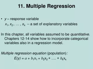
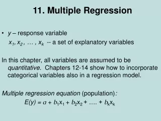
Estimated Multiple Regression Equation • Estimated Multiple Regression Equation ^ y = b0 + b1x1 + b2x2 + . . . + bpxp A simple random sample is used to compute sample statistics b0, b1, b2, . . . , bp that are used as the point estimators of the parameters b0, b1, b2, . . . , bp.
Least Squares Method • Least Squares Criterion
Multiple Regression Model Programmer Salary Survey A software firm collected data for a sample of 20 computer programmers. A suggestion was made that regression analysis could be used to determine if salary was related to the years of experience and the score on the firm’s programmer aptitude test. The years of experience, score on the aptitude test test, and corresponding annual salary ($1000s) for a sample of 20 programmers is shown on the next slide.
Multiple Regression Model Test Score Exper. (Yrs.) Exper. (Yrs.) Salary ($000s) Salary ($000s) Test Score 4 7 1 5 8 10 0 1 6 6 78 100 86 82 86 84 75 80 83 91 9 2 10 5 6 8 4 6 3 3 88 73 75 81 74 87 79 94 70 89 38.0 26.6 36.2 31.6 29.0 34.0 30.1 33.9 28.2 30.0 24.0 43.0 23.7 34.3 35.8 38.0 22.2 23.1 30.0 33.0
Multiple Regression Model Suppose we believe that salary (y) is related to the years of experience (x1) and the score on the programmer aptitude test (x2) by the following regression model: y = 0 + 1x1 + 2x2 + where y = annual salary ($000) x1 = years of experience x2 = score on programmer aptitude test
Solving for the Estimates of 0, 1, 2 Salary = 3.174 + 1.4039YearsExp + 0.25089ApScore Note: Predicted salary will be in thousands of dollars.
Multiple Coefficient of Determination • Relationship Among SST, SSR, SSE SST = SSR + SSE = + where: SST = total sum of squares SSR = sum of squares due to regression SSE = sum of squares due to error
SSR, SSE, and SST SSR SST SSE
Multiple Coefficient of Determination R2 = SSR/SST
Adjusted Multiple Coefficient of Determination Where p is the number of independent variables in the regression equation.
Testing for Significance: F Test The F test is used to determine whether a significant relationship exists between the dependent variable and the set of all the independent variables. The F test is referred to as the test for overall significance.
Testing for Significance: F Test H0: 1 = 2 = . . . = p = 0 Ha: One or more of the parameters is not equal to zero. Hypotheses F = MSR/MSE Test Statistics Rejection Rule Reject H0 if p-value <a or if F > F , where F is based on an F distribution with p d.f. in the numerator and n - p - 1 d.f. in the denominator.
F Test for Overall Significance Say a=0.05, is the regression significant overall?
Testing for Significance: t Test The t test is used to determine whether each of the individual independent variables is significant. A separate t test is conducted for each of the independent variables in the model. We refer to each of these t tests as a test for individual significance.
Testing for Significance: t Test Hypotheses Test Statistics Rejection Rule Reject H0 if p-value <a or if t< -tor t>twhere t is based on a t distribution with n - p - 1 degrees of freedom.
t Test for Significance of Individual Parameters Say a=0.05, which parameters are significant?
Multicollinearity The term multicollinearity refers to the correlation among the independent variables. When the independent variables are highly correlated, it is not possible to determine the separate effect of any particular independent variable on the dependent variable. Every attempt should be made to avoid including independent variables that are highly correlated.
Multicollinearity • The Variance Inflation Factor (VIF) measures how much the variance of the coefficient for an independent variable is inflated by one or more of the other independent variables. • This inflation of the variance means that the independent variable is highly correlated with at least one other independent variable. • VIF around 1 = no multicollinearity (good) • VIF much greater than 1 = multicollinearity (bad) • “much greater” is subjective!
Multicollinearity • VIF values not available in Excel • MiniTab:
Using the Estimated Regression Equationfor Estimation and Prediction The procedures for estimating the mean value of y and predicting an individual value of y in multiple regression are similar to those in simple regression. We substitute the given values of x1, x2, . . . , xp into the estimated regression equation and use the corresponding value of y as the point estimate.
Categorical Independent Variables In many situations we must work with categorical independent variablessuch as gender (male, female), method of payment (cash, check, credit card), etc. For example, x2 might represent gender where x2 = 0 indicates male and x2 = 1 indicates female. In this case, x2 is called a dummy or indicator variable.
Categorical Independent Variables The years of experience, the score on the programmer aptitude test, whether the individual has a relevant graduate degree, and the annual salary ($000) for each of the sampled 20 programmers are shown on the next slide. Programmer Salary Survey As an extension of the problem involving the computer programmer salary survey, suppose that management also believes that the annual salary is related to whether the individual has a graduate degree in computer science or information systems.
Categorical Independent Variables Exper. (Yrs.) Test Score Salary ($000s) Exper. (Yrs.) Test Score Salary ($000s) Degr. Degr. 4 7 1 5 8 10 0 1 6 6 78 100 86 82 86 84 75 80 83 91 No Yes No Yes Yes Yes No No No Yes 9 2 10 5 6 8 4 6 3 3 88 73 75 81 74 87 79 94 70 89 Yes No Yes No No Yes No Yes No No 38.0 26.6 36.2 31.6 29.0 34.0 30.1 33.9 28.2 30.0 24.0 43.0 23.7 34.3 35.8 38.0 22.2 23.1 30.0 33.0 If grad degree, Degr = 1. If no grad degree, Degr = 0.
Categorical Independent Variables Exper. (Yrs.) Test Score Salary ($000s) Exper. (Yrs.) Test Score Salary ($000s) Degr. Degr. 4 7 1 5 8 10 0 1 6 6 78 100 86 82 86 84 75 80 83 91 0 1 0 1 1 1 0 0 0 1 9 2 10 5 6 8 4 6 3 3 88 73 75 81 74 87 79 94 70 89 1 0 1 0 0 1 0 1 0 0 38.0 26.6 36.2 31.6 29.0 34.0 30.1 33.9 28.2 30.0 24.0 43.0 23.7 34.3 35.8 38.0 22.2 23.1 30.0 33.0
^ y = b0 + b1x1 +b2x2 + b3x3 where: y = annual salary ($1000) x1 = years of experience x2 = score on programmer aptitude test x3 = 0 if individual does not have a graduate degree 1 if individual does have a graduate degree ^ Estimated Regression Equation x3 is a dummy variable
More Complex Categorical Variables If a categorical variable has k levels, k - 1 dummy variables are required, with each dummy variable being coded as 0 or 1. For example, a variable with levels A, B, and C could be represented by x1 and x2 values of (0, 0) for A, (1, 0) for B, and (0,1) for C. Care must be taken in defining and interpreting the dummy variables.
Highest Degree x1 x2 Bachelor’s 0 0 Master’s 1 0 Ph.D. 0 1 More Complex Categorical Variables For example, a variable indicating level of education could be represented by x1 and x2 values as follows:
Assumptions About the Error Term The error is a random variable with mean of zero. The variance of , denoted by 2, is the same for all values of the independent variables. The values of are independent. The error is a normally distributed random variable reflecting the deviation between the y value and the expected value of y given by 0 + 1x1 + 2x2 + . . + pxp.
Standardized Residual Plot Against • Standardized residuals are frequently used in residual plots for purposes of: • Identifying outliers (typically, standardized residuals < -2 or > +2) • Providing insight about the assumption that the error term e has a normal distribution