
2. Compression Algorithms for Multimedia Data Streams
E N D
Presentation Transcript
2. Compression Algorithms for MultimediaData Streams • 2.1 Fundamentals of Data Compression • 2.2 Compression of Still Images • 2.3 Video Compression • 2.4 Audio Compression
2.1 Fundamentals of Data Compression • Motivation: huge data volumes • Text1 page with 80 characters/line and 64 lines/page and 1 byte/char results in 80 * 64 * 1 * 8 = 41 kbit/page • Still image24 bits/pixel, 512 x 512 pixel/image results in 512 x 512 x 24 = ca. 6 Mbit/image • AudioCD quality, sampling rate 44,1 KHz, 16 bits per sample results in 44,1 x 16 = 706 kbit/s. Stereo: 1,412 Mbit/s • VideoFull-size frame 1024 x 768 pixel/frame, 24 bits/pixel, 30 frames/s results in 1024 x 768 x 24 x 30 = 566 Mbit/s.More realistic: 360 x 240 pixel/frame, 360 x 240 x 24 x 30 = 60 Mbit/s • => Storage and transmission of multimedia streams require compression.
Principles of Data Compression • 1. Lossless Compression • The original object can be reconstructed perfectly • Compression rates of 2:1 to 50:1 are typical • Example: Huffman coding • 2. Lossy Compression • There is a difference between the original object and the reconstructed object. • Physiological and psychological properties of the ear and eye can be taken into account. • Higher compression rates are possible than with lossless compression (typically up to 100:1).
Simple Lossless Algorithms: Pattern Substitution • Example 1: ABC -> 1; EE -> 2 Example 2: Note that in this example both algorithms lead to the same compression rate.
Run Length Coding • Principle • Replace all repetitions of the same symbol in the text (”runs“) by a repetition counter and the symbol. • Example • Text: • AAAABBBAABBBBBCCCCCCCCDABCBAABBBBCCD • Encoding: • 4A3B2A5B8C1D1A1B1C1B2A4B2C1D • As we can see, we can only expect a good compression rate when long runs occur frequently. • Examples are long runs of blanks in text documents, leading zeroes in numbers or strings of „white“ in gray-scale images.
Run Length Coding for Binary Files • When dealing with binary files we are sure that a run of “1“s is always followed by a run of “0“s and vice versa. It is thus sufficient to store the repetition counters only! • Example • 000000000000000000000000000011111111111111000000000 28 14 9 • 000000000000000000000000001111111111111111110000000 26 18 7 • 000000000000000000000001111111111111111111111110000 23 24 4 • 000000000000000000000011111111111111111111111111000 22 26 3 • 000000000000000000001111111111111111111111111111110 20 30 1 • 000000000000000000011111110000000000000000001111111 19 7 18 7 • 000000000000000000011111000000000000000000000011111 19 5 22 5 • 000000000000000000011100000000000000000000000000111 19 3 26 3 • 000000000000000000011100000000000000000000000000111 19 3 26 3 • 000000000000000000011100000000000000000000000000111 19 3 26 3 • 000000000000000000011100000000000000000000000000111 19 3 26 3 • 000000000000000000001111000000000000000000000001110 20 4 23 3 1 • 000000000000000000000011100000000000000000000111000 22 3 20 3 3 • 011111111111111111111111111111111111111111111111111 1 50 • 011111111111111111111111111111111111111111111111111 1 50 • 011111111111111111111111111111111111111111111111111 1 50 • 011111111111111111111111111111111111111111111111111 1 50 • 011111111111111111111111111111111111111111111111111 1 50 • 011000000000000000000000000000000000000000000000011 1 2 46 2
Run Length Coding, Legal Issues • Beware of the patent trap! • Runlength encoding of the type (length, character) • US Patent No: 4,586,027 • Title: Method and system for data compression and restoration • Filed: 07-Aug-1984 • Granted: 29-Apr-1986 • Inventor: Tsukimaya et al. • Assignee: Hitachi • Runlength encoding (length [<= 16], character) • Number: 4,872,009 • Title: Method and apparatus for data compression and restoration • Filed: 07-Dec-1987 • Granted: 03-Oct-1989 • Inventor: Tsukimaya et al. • Assignee: Hitachi
Variable Length Coding • Classical character codes use the same number of bits for each character. When the frequency of occurrence is different for different characters, we can use fewer bits for frequent characters and more bits for rare characters. • Example • Code 1: A B C D E ... • 1 2 3 4 5 (binary) • Encoding of ABRACADABRA with constant bit length (= 5 Bits): • 0000100010100100000100011000010010000001000101001000001 • Code 2: A B R C D • 0 1 01 10 11 • Encoding:0 1 01 0 10 0 11 0 1 010
Delimiters • Code 2 can only be decoded unambiguously when delimiters are stored with the codewords. This can increase the size of the encoded string considerably. • Idea • No code word should be the prefix of another codeword! We will then no longer need delimiters. • Code 3: Encoded string: 1100011110101110110001111
Representation as a TRIE • An obvious method to represent such a code as a TRIE. In fact, any TRIE with M leaf nodes can be used to represent a code for a string containing M different characters. • The figure on the next page shows two codes which can be used for ABRACADABRA. The code for each character is represented by the path from the root of the TRIE to that character where “0“ goes to the left, “1“ goes to the right, as is the convention for TRIEs. • The TRIE on the left corresponds to the encoding of ABRACADABRA on the previous page, the TRIE on the right generates the following encoding: • 01101001111011100110100 • which is two bits shorter.
Two Tries for our Example • The TRIE representation guarantees indeed that no codeword is the prefix of another codeword. Thus the encoded bit string can be uniquely decoded.
Huffman Code • Now the question arises how we can find the best variable-length code for given character frequencies (or probabilities). The algorithm that solves this problem was found by David Huffman in 1952. • Algorithm Generate-Huffman-Code • Determine the frequencies of the characters and mark the leaf nodes of a binary tree (to be built) with them. • Out of the tree nodes not yet marked as DONE, take the two with the smallest frequencies and compute their sum. • Create a parent node for them and mark it with the sum. Mark the branch to the left son with 0, the one to the right son with 1. • Mark the two son nodes as DONE. When there is only one node not yet marked as DONE, stop (the tree is complete). Otherwise, continue with step 2.
Huffman Code, Example • Probabilities of the characters: • p(A) = 0.3; p(B) = 0.3; p(C) = 0.1; p(D) = 0.15; p(E) = 0.15 1 11 A 30% 1 60% 10 B 30% 0 100% 1 C 10% 011 1 25% 010 D 15% 40% 0 0 00 E 15% 0
Huffman Code, why is it optimal? • Characters with higher probabilities are closer to the root of the tree and thus have shorter codeword lengths; thus it is a good code. It is even the best possible code! • Reason: • The length of an encoded string equals the weighted outer path length of the Huffman tree. • To compute the “weighted outer path length“ we first compute the product of the weight (frequency counter) of a leaf node with its distance from the root. We then compute the sum of all these values over the leaf nodes. This is obviously the same as summing up the products of each character‘s codeword length with its frequency of occurrence. • No other tree with the same frequencies attached to the leaf nodes has a smaller weighted path length than the Huffman tree.
Sketch of the Proof • With a similar construction process, another tree could be built but without always combining the two nodes with the minimal frequencies. We can show by induction that no other such strategy will lead to a smaller weighted outer path length than the one that combines the minimal values in each step.
Decoding Huffman Codes (1) • An obvious possibility is to use the TRIE: • Read the input stream sequentially and traverse the TRIE until a leaf node is reached. • When a leaf node is reached, output the character attached to it. • To decode the next bit, start againat the root of the TRIE. Observation The input bit rate is constant, the output character rate is variable.
Decoding Huffman Codes (2) • As an alternative we can use a decoding table. • Creation of the decoding table: • If the longest codeword has L bits, the table has 2L entries. • Let ci be the codeword for character si. Let ci have li bits. We then create 2L-li entries in the table. In each of these entries the first li bits are equal to ci, and the remaining bits take on all possible L-li binary combinations. • At all these addresses of the table we enter si as the character recognized, and we remember li as the length of the codeword.
Decoding Huffman Codes (3) • Algorithm Table-Based Huffman Decoder • Read L bits from the input stream into a buffer. • Use the buffer as the address into the table and output the recognized character si. • Remove the first li bits from the buffer and pull in the next li bits from the input bit stream. • Continue with step 2. • Observation • Table-based Huffman decoding is fast. • The output character rate is constant, the input bit rate is variable.
Huffman Code, Comments • A very good code for many practical purposes. • Can only be used when the frequencies (or probabilities) of the characters are known in advance. • Variation: Determine the character frequencies separately for each new document and store/transmit the code tree/table with the data. • Note that a loss in “optimality“ comes from the fact that each character must be encoded with a fixed number of bits, and thus the codeword lengths do not match the frequencies exactly (consider a code for three characters A, B and C, each occurring with a frequency of 33 %).
Lempel-Ziv Code • Lempel-Ziv codes are an example of the large group of dictionary-based codes. • Dictionary: A table of character strings which is used in the encoding process. • Example • The word “lecture“ is found on page x4, line y4 of the dictionary. It can thus be en-coded as (x4,y4). • A sentence such as „this is a lecture“ could perhaps be encoded as a sequence of tuples (x1,y1) (x2,y2) (x3,y3) (x4,y4).
Dictionary-Based Coding Techniques • Static techniques • The dictionary exists before a string is encoded. It is not changed, neither in the en-coding nor in the decoding process. • Dynamic techniques • The dictionary is created “on the fly“ during the encoding process, at the sending (and sometimes also at the receiving) side. • Lempel and Ziv have proposed an especially brilliant dynamic, dictionary-based technique (1977). Variations of this techniques are used very widely today for lossless compression. An example is LZW (Lempel/Ziv/Welch) which is invoked with the Unix compress command. • The well-known TIFF format (Tag Image File Format) is also based on Lempel-Ziv coding.
Ziv-Lempel Coding, the Principle • Idea (pretty bright!) • The current piece of the message can be encoded as a reference to an earlier (iden-tical) piece of the message. This reference will usually be shorter than the piece itself. As the message is processed, the dictionary is created dynamically. • LZW Algorithm • InitializeStringTable(); • WriteCode(ClearCode); • = the empty string; • for each character in string { • K = GetNextCharacter(); • if + K is in the string table { • =+K /* string concatenation*/ • } else { • WriteCode(CodeFromString()); • AddTableEntry(+K); • =K • } • } • WriteCode(CodeFromString());
LZW, Example 1, Encoding • Alphabet: {A, B, C} Message: ABA BCB A B A B 1 2 4 3 5 8 Encoded message: A A AB B BA A A ? B AB AB C C ABC AB CB B 4 BA BA BA 5 ABC 6 BAB B CB BA BA 7 BAB BAB BAB 8
LZW Algorithm: Decoding (1) • Note that the decoding algorithm also creates the dictionary dynamically, the dictio-nary is not transmitted! • While((Code=GetNextCode() != EofCode){ • if (Code == ClearCode) • { • InitializeTable(); • Code = GetNextCode(); • if (Code==EofCode) • break; • WriteString(StringFromCode(Code)); • OldCode = Code; • } /* end of ClearCode case */ • else • { • if (IsInTable(Code)) • { • WriteString( StringFromCode(Code) ); • AddStringToTable(StringFromCode(OldCode)+ • FirstChar(StringFromCode(Code))); • OldCode = Code; • }
LZW Algorithm: Decoding (2) • else • {/* code is not in table */ • OutString = StringFromCode(OldCode) + • FirstChar(StringFromCode(OldCode))); • WriteString(OutString); • AddStringToTable(OutString); • OldCode = Code; • } • } • }
LZW, Example 2, Decoding 1 2 1 3 5 1 • Alphabet: {A, B, C,D} • Decoded Message: Transmitted Code: C A AB A A B 1 1 2 2 1 1 3 3 5 5 AB 5 1 1 BA 6 AC 7 CA 8 ABA 9
LZW, Properties • The dictionary is created dynamically during the encoding and decoding process. It is neither stored nor transmitted! • The dictionary adapts dynamically to the properties of the character string. • With length N of the original message, the encoding process is of complexity O(N). With length M of the encoded message, the decoding process is of complexity O(M). These are thus very efficient processes. Since several characters of the input alphabet are combined into one character of the code, M <= N.
Typical Compression Rates • Typical examples of file sizes in % of the original size
Arithmetic Coding • From an information theory point of view, the Huffman code is not quite optimal since a codeword must always consist of an integer number of bits even if this does not correspond exactly to the frequency of occurrence of the character. Arithmetic coding solves this problem. • Idea • An entire message is represented by a floating point number out of the interval [0,1). For this purpose the interval [0,1) is repeatedly subdivided according to the frequency of the next symbol. Each new sub-interval represents one symbol. When the process is completed the shortest floating point number contained in the target interval is cho-sen as the representative for the message.
Arithmetic Coding, the Algorithm • Algorithm Arithmetic Encoding • Begin in front of the first character of the input stream, with the current interval set to [0,1). • Read the next character from the input stream. Subdivide the current interval according to the frequencies of all characters of the alphabet. Select the subinterval corresponding to the current character as the next current interval. • If you reach the end of the input stream or the end symbol, go to step 3. Otherwise go to step 1. • From the current (final) interval, select the floating point number that you can represent in the computer with the smallest number of bits. This number is the encoding of the string.
Arithmetic Coding, the Decoding Algorithm • Algorithm Arithmetic Decoding • Subdivide the interval [0,1) according to the character frequencies, as described in the encoding algorithm, up to the maximum size of a message. • The encoded floating point number uniquely identifies one particular subinterval. • This subinterval uniquely identifies one particular message. Output the message.
0 0,2 0,5 1 A B C 0 0,04 0,1 0,2 A B C 0,1 0,12 0,15 0,2 A B C Arithmetic Coding, Example • Alphabet = {A,B,C} • Frequencies (probabilities): p(A) = 0.2; p(B) = 0.3; p(C) = 0.5 • Messages: ACB AAB (maximum size of a messe is 3). • Encoding of the first block ACB: Final interval:[0.12; 0.15) choose e.g. 0.125
Arithmetic Coding, Implementation (1) • So far we dealt with real numbers of (theoretically) infinite precision. How do we actually encode a message with many characters (say, several megabytes)? • If character ‘A’ occurs with a probability of 20%, the number of digits for coding con-secutive ‘A’s grows very fast: • First A < 0.2, second A < 0.04, third A < 0.008, 0.0016, 0.00032, 0.000064 and so on. • Let us assume, that our processor has 8-bit-wide registers. (decimal 0) 0.00000000 (0.2 x 255=51) 0.00110011 (0.5 x 255=127) 0.01111111 (decimal 255) 0.11111111 A B C 0,2 0,5 Note: We do not store or transmit the “0.” from the beginning since it is redundant. Advantage: We have a binary fixed-point arithmetic representation of fractions, and we can compute them in the register of the processor.
Arithmetic Coding, Implementation (2) • Disadvantage: Even when using 32-bit or 64-bit CPU registers we can only encode a few characters at a time. • Solution: When our interval gets smaller and smaller, we will obtain a growing number of leading bits which have settled (they will never change). So we will transmit them to the receiver and shift them out of our register to gain room for new bits. • Example: Interval of first A = [ 0.00000000 , 0.00110011 ] • No matter which characters follow, the most significant two zeros from the lower and the upper bound will never change. So we store or transmit them and shift the rest two digits to the left. As a consequence we gain two new least significant digits: • A=[ 0.000000?? , 0.110011?? ]
Arithmetic Coding, Implementation (3) • A=[ 0.000000?? , 0.110011?? ] • How do we initialize the new digits prior to the ongoing encoding? • Obviously, we want to keep the interval as large as possible. This is achieved by filling the lower bound with 0-bits and the upper bound with 1-bits. • Anew=[ 0.00000000 , 0.11001111 ] • Note that always adding 0-bits to the lower bound and 1-bits to the upper bound intro-duces a mistake because the size of the interval does not exactly correspond to the probability of character ‘A’. However, we will not get into trouble if the encoding and the decoding side make the same mistake.
Arithmetic Coding, Properties • The encoding depends on the probabilities (frequency of occurrences) of the char-acters. The higher the frequency, the larger the subinterval, and the smaller the number of bits needed to represent it. • The code length reaches the theoretical optimum: The number of bits used for each character need not be an integer. It can approach the real probability better than with the Huffman code. • We always need a terminal symbol to stop the encoding process. Problem: One bit error destroys the entire message!