Download

1 / 37
380 likes | 649 Views
Mining Frequent Patterns, Association, and Correlations (cont.) Pertemuan 06. Matakuliah : M0614 / Data Mining & OLAP Tahun : Feb - 2010. Learning Outcomes. Pada akhir pertemuan ini, diharapkan mahasiswa akan mampu :

E N D
Mining Frequent Patterns, Association, and Correlations (cont.)Pertemuan 06 Matakuliah : M0614 / Data Mining & OLAP Tahun : Feb - 2010
Learning Outcomes Pada akhir pertemuan ini, diharapkan mahasiswa akan mampu : • Mahasiswa dapat menggunakan teknik analisis mining frequent pattern dan association and correlations pada data mining. (C3) 3
Acknowledgments These slides have been adapted from Han, J., Kamber, M., & Pei, Y. Data Mining: Concepts and Technique. Bina Nusantara
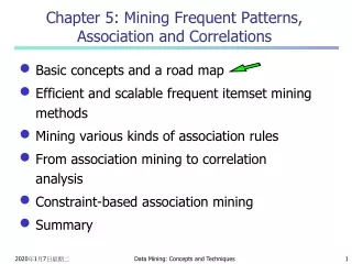
Mining various kind of association rules From association to correlation analysis Constraint-based association mining Summary Outline Materi 5 Bina Nusantara
Mining Various Kinds of Association Rules • Mining multilevel association • Miming multidimensional association • Mining quantitative association • Mining interesting correlation patterns
uniform support reduced support Level 1 min_sup = 5% Milk [support = 10%] Level 1 min_sup = 5% Level 2 min_sup = 5% 2% Milk [support = 6%] Skim Milk [support = 4%] Level 2 min_sup = 3% Mining Multiple-Level Association Rules • Items often form hierarchies • Flexible support settings • Items at the lower level are expected to have lower support • Exploration of shared multi-level mining
Multi-level Association: Redundancy Filtering • Some rules may be redundant due to “ancestor” relationships between items • Example • milk wheat bread [support = 8%, confidence = 70%] • 2% milk wheat bread [support = 2%, confidence = 72%] • We say the first rule is an ancestor of the second rule • A rule is redundant if its support is close to the “expected” value, based on the rule’s ancestor
Mining Multi-Dimensional Association • Single-dimensional rules: buys(X, “milk”) buys(X, “bread”) • Multi-dimensional rules: 2 dimensions or predicates • Inter-dimension assoc. rules (no repeated predicates) age(X,”19-25”) occupation(X,“student”) buys(X, “coke”) • hybrid-dimension assoc. rules (repeated predicates) age(X,”19-25”) buys(X, “popcorn”) buys(X, “coke”) • Categorical Attributes: finite number of possible values, no ordering among values—data cube approach • Quantitative Attributes: Numeric, implicit ordering among values—discretization, clustering, and gradient approaches
Mining Quantitative Associations Techniques can be categorized by how numerical attributes, such as ageorsalary are treated • Static discretization based on predefined concept hierarchies (data cube methods) • Dynamic discretization based on data distribution (quantitative rules) • Clustering: Distance-based association One dimensional clustering then association • Deviation: Sex = female => Wage: mean=$7/hr (overall mean = $9)
() (age) (income) (buys) (age, income) (age,buys) (income,buys) (age,income,buys) Static Discretization of Quantitative Attributes • Discretized prior to mining using concept hierarchy. • Numeric values are replaced by ranges • In relational database, finding all frequent k-predicate sets will require k or k+1 table scans • Data cube is well suited for mining • The cells of an n-dimensional cuboid correspond to the predicate sets • Mining from data cubescan be much faster
Quantitative Association Rules • Numeric attributes are dynamically discretized • Such that the confidence or compactness of the rules mined is maximized • 2-D quantitative association rules: Aquan1 Aquan2 Acat • Cluster adjacent association rules to form general rules using a 2-D grid • Example: age(X, “34-35”) income(X, “30-50K”) buys(X, “high resolution TV”)
Mining Other Interesting Patterns • Flexible support constraints • Some items (e.g., diamond) may occur rarely but are valuable • Customized supmin specification and application • Top-K closed frequent patterns • Hard to specify supmin, but top-kwith lengthmin is more desirable • Dynamically raise supmin in FP-tree construction and mining, and select most promising path to mine
From association mining to correlation analysis : Interestingness Measure: Correlations (Lift) • play basketball eat cereal [40%, 66.7%] is misleading • The overall % of students eating cereal is 75% > 66.7%. • play basketball not eat cereal [20%, 33.3%] is more accurate, although with lower support and confidence • Measure of dependent/correlated events: lift
Constraint-based (Query-Directed) Mining • Finding all the patterns in a database autonomously? — unrealistic! • The patterns could be too many but not focused! • Data mining should be an interactive process • User directs what to be mined using a data mining query language(or a graphical user interface) • Constraint-based mining • User flexibility: providesconstraints on what to be mined • System optimization: explores such constraints for efficient mining — constraint-based mining: constraint-pushing, similar to push selection first in DB query processing • Note: still find all the answers satisfying constraints, not finding some answers in “heuristic search”
Constraints in Data Mining • Knowledge type constraint: • classification, association, etc. • Data constraint— using SQL-like queries • find product pairs sold together in stores in Chicago in Dec.’02 • Dimension/level constraint • in relevance to region, price, brand, customer category • Rule (or pattern) constraint • small sales (price < $10) triggers big sales (sum > $200) • Interestingness constraint • strong rules: min_support 3%, min_confidence 60%
Constraint-Based Frequent Pattern Mining • Classification of constraints based on their constraint-pushing capabilities • Anti-monotonic: If constraint c is violated, its further mining can be terminated • Monotonic: If c is satisfied, no need to check c again • Data anti-monotonic: If a transaction t does not satisfy c, t can be pruned from its further mining • Succinct: c must be satisfied, so one can start with the data sets satisfying c • Convertible: c is not monotonic nor anti-monotonic, but it can be converted into it if items in the transaction can be properly ordered
Anti-Monotonicity in Constraint Pushing TDB (min_sup=2) • A constraint C is antimonotone if the super pattern satisfies C, all of its sub-patterns do so too • In other words, anti-monotonicity: If an itemset S violates the constraint, so does any of its superset • Ex. 1. sum(S.price) v is anti-monotone • Ex. 2.range(S.profit) 15 is anti-monotone • Itemset ab violates C • So does every superset of ab • Ex. 3. sum(S.Price) v is not anti-monotone • Ex. 4. support count is anti-monotone: core property used in Apriori
Monotonicity for Constraint Pushing TDB (min_sup=2) • A constraint C is monotone if the pattern satisfies C, we do not need to check C in subsequent mining • Alternatively, monotonicity: If an itemset S satisfies the constraint, so does any of its superset • Ex. 1. sum(S.Price) v is monotone • Ex. 2. min(S.Price) v is monotone • Ex. 3. C: range(S.profit) 15 • Itemset ab satisfies C • So does every superset of ab
Data Antimonotonicity: Pruning Data Space TDB (min_sup=2) • A constraint c is data antimonotone if for a pattern p cannot satisfy a transaction t under c, p’s superset cannot satisfy t under c either • The key for data antimonotone is recursive data reduction Ex. 1. sum(S.Price) v is data antimonotone Ex. 2. min(S.Price) v is data antimonotone Ex. 3. C: range(S.profit) 25 is data antimonotone • Itemset {b, c}’s projected DB: • T10’: {d, f, h}, T20’: {d, f, g, h}, T30’: {d, f, g} • since C cannot satisfy T10’, T10’ can be pruned
Succinctness • Succinctness: • Given A1, the set of items satisfying a succinctness constraint C, then any set S satisfying C is based on A1 , i.e., S contains a subset belonging to A1 • Idea: Without looking at the transaction database, whether an itemset S satisfies constraint C can be determined based on the selection of items • min(S.Price) v is succinct • sum(S.Price) v is not succinct • Optimization: If C is succinct, C is pre-counting pushable
The Apriori Algorithm — Example Database D L1 C1 Scan D C2 C2 L2 Scan D L3 C3 Scan D
Naïve Algorithm: Apriori + Constraint Database D L1 C1 Scan D C2 C2 L2 Scan D L3 C3 Constraint: Sum{S.price} < 5 Scan D
The Constrained Apriori Algorithm: Push a Succinct Constraint Deep Database D L1 C1 Scan D C2 C2 L2 Scan D not immediately to be used L3 C3 Constraint: min{S.price } <= 1 Scan D
The Constrained FP-Growth Algorithm: Push a Succinct Constraint Deep FP-Tree Remove infrequent length 1 1-Projected DB No Need to project on 2, 3, or 5 Constraint: min{S.price } <= 1
The Constrained FP-Growth Algorithm: Push a Data Antimonotonic Constraint Deep Remove from data FP-Tree Single branch, we are done Constraint: min{S.price } <= 1
The Constrained FP-Growth Algorithm: Push a Data Antimonotonic Constraint Deep FP-Tree B-Projected DB Recursive Data Pruning B FP-Tree • Single branch: • bcdfg: 2 Constraint: range{S.price } > 25 min_sup >= 2
Converting “Tough” Constraints TDB (min_sup=2) • Convert tough constraints into anti-monotone or monotone by properly ordering items • Examine C: avg(S.profit) 25 • Order items in value-descending order • <a, f, g, d, b, h, c, e> • If an itemset afb violates C • So does afbh, afb* • It becomes anti-monotone!
Strongly Convertible Constraints • avg(X) 25 is convertible anti-monotone w.r.t. item value descending order R: <a, f, g,d, b, h, c, e> • If an itemset af violates a constraint C, so does every itemset with af as prefix, such as afd • avg(X) 25 is convertible monotone w.r.t. item value ascending order R-1: <e, c, h, b, d, g, f, a> • If an itemset d satisfies a constraint C, so does itemsets df and dfa, which having d as a prefix • Thus, avg(X) 25 is strongly convertible
Can Apriori Handle Convertible Constraints? • A convertible, not monotone nor anti-monotone nor succinct constraint cannot be pushed deep into the an Apriori mining algorithm • Within the level wise framework, no direct pruning based on the constraint can be made • Itemset df violates constraint C: avg(X) >= 25 • Since adf satisfies C, Apriori needs df to assemble adf, df cannot be pruned • But it can be pushed into frequent-pattern growth framework!
Mining With Convertible Constraints • C: avg(X) >= 25, min_sup=2 • List items in every transaction in value descending order R: <a, f, g, d, b, h, c, e> • C is convertible anti-monotone w.r.t. R • Scan TDB once • remove infrequent items • Item h is dropped • Itemsets a and f are good, … • Projection-based mining • Imposing an appropriate order on item projection • Many tough constraints can be converted into (anti)-monotone TDB (min_sup=2)
Handling Multiple Constraints • Different constraints may require different or even conflicting item-ordering • If there exists an order R s.t. both C1 and C2 are convertible w.r.t. R, then thereis no conflict between the two convertible constraints • If there exists conflict on order of items • Try to satisfy one constraint first • Then using the order for the other constraint to mine frequent itemsets in the corresponding projected database
Monotone Antimonotone Strongly convertible Succinct Convertible anti-monotone Convertible monotone Inconvertible A Classification of Constraints
Frequent-Pattern Mining: Summary • Frequent pattern mining—an important task in data mining • Scalable frequent pattern mining methods • Apriori (Candidate generation & test) • Projection-based (FPgrowth, CLOSET+, ...) • Vertical format approach (CHARM, ...) • Mining a variety of rules and interesting patterns • Constraint-based mining • Mining sequential and structured patterns • Extensions and applications
Dilanjutkan ke pert. 07 Classification and Prediction