Download
1 / 54
540 likes | 697 Views
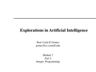
CS344 : Introduction to Artificial Intelligence. Pushpak Bhattacharyya CSE Dept., IIT Bombay Lecture 28- PAC and Reinforcement Learning. U Universe. C. h. C h = Error region. +. P(C h ) <= Є. +. accuracy parameter. Prob. distribution. +.

E N D
CS344 : Introduction to Artificial Intelligence Pushpak BhattacharyyaCSE Dept., IIT Bombay Lecture 28- PAC and Reinforcement Learning
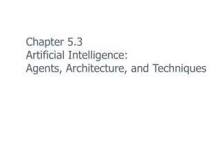
U Universe C h C h = Error region + P(C h ) <= Є + accuracy parameter Prob. distribution
+ Learning Means the following Should happen: Pr(P(c h) <= Є) >= 1- δ PAC model of learning correct. Probably Approximately Correct
y A B - + - - - - - + - - + - - - C - D x IIT Bombay
Algo: 1. Ignore –ve example. 2. Find the closest fitting axis parallel rectangle for the data.
Pr(P(c h) <= Є ) >= 1- δ y + c C h + A B - - - - - - + + - - + h - - - C - D Case 1: If P([]ABCD) < Є than the Algo is PAC. x
Case 2 p([]ABCD) > Є y A B Top - - - - - - - - Right Left - - - C - D Case 2: x Bottom P(Top) = P(Bottom) = P(Right) = P(Left) = Є/4
Let # of examples = m. • Probability that a point comes from top = Є/4 • Probability that none of the m example come from top = (1- Є/4)m IIT Bombay
Probability that none of m examples come from one of top/bottom/left/right = 4(1 - Є/4)m Probability that at least one example will come from the 4 regions = 1- 4(1 - Є/4)m
This fact must have probability greater than or equal to 1- δ 1-4 (1 - Є/4 )m >1- δ or 4(1 - Є/4 )m < δ
(1 - Є/4)m < e(-Єm/4) We must have 4 e(-Єm/4) < δ Or m > (4/Є) ln(4/δ)
Lets say we want 10% error with 90% confidence M > ((4/0.1) ln (4/0.1)) Which is nearly equal to 200
VC-dimension Gives a necessary and sufficient condition for PAC learnability.
C C1 C3 Def:- Let C be a concept class, i.e., it has members c1,c2,c3,…… as concepts in it. C2
Let S be a subset of U (universe). Now if all the subsets of S can be produced by intersecting with Cis, then we say C shatters S.
The highest cardinality set S that can be shattered gives the VC-dimension of C. VC-dim(C)= |S| VC-dim: Vapnik-Cherronenkis dimension.
y 2 – Dim surface C = { half planes} x IIT Bombay
y S1= { a } {a}, Ø a x |s| = 1 can be shattered IIT Bombay
y S2= { a,b } {a,b}, {a}, {b}, Ø b a x |s| = 2 can be shattered IIT Bombay
y S3= { a,b,c } b a c x |s| = 3 can be shattered IIT Bombay
y S4= { a,b,c,d } A B C D x |s| = 4 cannot be shattered IIT Bombay
Fundamental Theorem of PAC learning (Ehrenfeuct et. al, 1989) • A Concept Class C is learnable for all probability distributions and all concepts in C if and only if the VC dimension of C is finite • If the VC dimension of C is d, then…(next page) IIT Bombay
Fundamental theorem (contd) (a) for 0<ε<1 and the sample size at least max[(4/ε)log(2/δ), (8d/ε)log(13/ε)] any consistent function A:ScC is a learning function for C (b) for 0<ε<1/2 and sample size less than max[((1-ε)/ ε)ln(1/ δ), d(1-2(ε(1- δ)+ δ))] No function A:ScH, for any hypothesis space is a learning function for C. IIT Bombay
Paper’s • 1. A theory of the learnable, Valiant, LG (1984), Communications of the ACM 27(11):1134 -1142. • 2. Learnability and the VC-dimension, A Blumer, A Ehrenfeucht, D Haussler, M Warmuth - Journal of the ACM, 1989. Book Computational Learning Theory, M. H. G. Anthony, N. Biggs, Cambridge Tracts in Theoretical Computer Science, 1997.
Introduction • Reinforcement Learning is a sub-area of machine learning concerned with how an agent ought to take actions in an environment so as to maximize some notion of long-term reward.
Constituents • In RL no correct/incorrrect input/output are given. • Feedback for the learning process is called 'Reward' or 'Reinforcement' • In RL we examine how an agent can learn from success and failure, reward and punishment
The RL framework • Environment is depicted as a finite-state Markov Decision process.(MDP) • Utility of a state U[i] gives the usefulness of the state • The agent can begin with knowledge of the environment and the effects of its actions; or it will have to learn this model as well as utility information.
The RL problem • Rewards can be received either in intermediate or a terminal state. • Rewards can be a component of the actual utility(e.g. Pts in a TT match) or they can be hints to the actual utility (e.g. Verbal reinforcements) • The agent can be a passive or an active learner
Passive Learning in a Known Environment In passive learning, the environment generates state transitions and the agent perceives them. Consider an agent trying to learn the utilities of the states shown below:
Passive Learning in a Known Environment • Agent can move {North, East, South, West} • Terminate on reading [4,2] or [4,3]
Passive Learning in a Known Environment Agent is provided: Mi j =a model given the probability of reaching from state i to state j
Passive Learning in a Known Environment • The object is to use this information about rewards to learn the expected utility U(i) associated with each nonterminal state i • Utilities can be learned using 3 approaches 1) LMS (least mean squares) 2) ADP (adaptive dynamic programming) 3) TD (temporal difference learning)
Passive Learning in a Known Environment LMS (Least Mean Square) Agent makes random runs (sequences of random moves) through environment [1,1]->[1,2]->[1,3]->[2,3]->[3,3]->[4,3] = +1 [1,1]->[2,1]->[3,1]->[3,2]->[4,2] = -1
Passive Learning in a Known Environment LMS • Collect statistics on final payoff for each state(eg. when on [2,3], how often reached +1 vs -1 ?) • Learner computes average for each state Probably converges to true expected value (utilities)
Passive Learning in a Known Environment LMS Main Drawback: - slow convergence - it takes the agent well over a 1000 training sequences to get close to the correct value
Passive Learning in a Known Environment ADP (Adaptive Dynamic Programming) Uses the value or policy iteration algorithm to calculate exact utilities of states given an estimated mode
Passive Learning in a Known Environment ADP In general: Un+1(i) = Un(i)+ ∑ Mij . Un(j) -Un(i) is the utility of state i after nth iteration -Initially set to R(i) - R(i) is reward of being in state i (often non zero for only a few end states) - Mij is the probability of transition from state i to j
Passive Learning in a Known Environment ADP Consider U(3,3) U(3,3) = 0.33 x U(4,3) + 0.33 x U(2,3) + 0.33 x U(3,2) = 0.33 x 1.0 + 0.33 x 0.0886 + 0.33 x -0.4430 = 0.2152
Passive Learning in a Known Environment ADP • makes optimal use of the local constraints on utilities of states imposed by the neighborhood structure of the environment • somewhat intractable for large state spaces
Passive Learning in a Known Environment TD (Temporal Difference Learning) The key is to use the observed transitions to adjust the values of the observed states so that they agree with the constraint equations
Passive Learning in a Known Environment TD Learning • Suppose we observe a transition from state i to state j U(i) = -0.5 and U(j) = +0.5 • Suggests that we should increase U(i) to make it agree better with it successor • Can be achieved using the following updating rule Un+1(i) = Un(i)+ a(R(i) + Un(j) –Un(i))
Passive Learning in a Known Environment TD Learning Performance: • Runs “noisier” than LMS but smaller error • Deal with observed states during sample runs (Not all instances, unlike ADP)
Passive Learning in an Unknown Environment LMS approach and TD approach operate unchanged in an initially unknown environment. ADP approach adds a step that updates an estimated model of the environment.
Passive Learning in an Unknown Environment ADP Approach • The environment model is learned by direct observation of transitions • The environment model M can be updated by keeping track of the percentage of times each state transitions to each of its neighbours
Passive Learning in an Unknown Environment ADP & TD Approaches • The ADP approach and the TD approach are closely related • Both try to make local adjustments to the utility estimates in order to make each state “agree” with its successors
Passive Learning in an Unknown Environment Minor differences : • TD adjusts a state to agree with its observed successor • ADP adjusts the state to agree with all of the successors Important differences : • TD makes a single adjustment per observed transition • ADP makes as many adjustments as it needs to restore consistency between the utility estimates U and the environment model M
Passive Learning in an Unknown Environment To make ADP more efficient : • directly approximate the algorithm for value iteration or policy iteration • prioritized-sweeping heuristic makes adjustments to states whose likely successors have just undergone a large adjustment in their own utility estimates Advantage of the approximate ADP : • efficient in terms of computation • eliminate long value iterations occur in early stage
Active Learning in an Unknown Environment An active agent must consider : • what actions to take • what their outcomes may be • how they will affect the rewards received