Download
1 / 46
530 likes | 778 Views
Radiative Transfer, Canopy Radiation and Turbulence. Paul Dirmeyer Center for Ocean-Land-Atmosphere Studies. Radiative Transfer. Energy transfer between the surface and adjacent matter (above and below) is accomplished by various mechanisms: Radiative transfer Light (visible radiation)

E N D
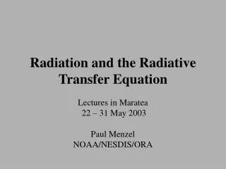
Radiative Transfer, Canopy Radiation and Turbulence Paul Dirmeyer Center for Ocean-Land-Atmosphere Studies CLIM 714 Land-Climate Interactions
Radiative Transfer Energy transfer between the surface and adjacent matter (above and below) is accomplished by various mechanisms: • Radiative transfer • Light (visible radiation) • Heat (thermal or infrared radiation) • Conduction to adjacent surfaces • Sensible heat (air above) • Heat diffusion (into the soil below) • Latent heating • Phase change of water (evaporation, transpiration, sublimation, melting) • Mass transport (interception, throughfall, infiltration) CLIM 714 Land-Climate Interactions
The Electromagnetic spectrum The chart below shows the common names given to regions of the electromagnetic spectrum, and their corresponding wavelengths. Given the speed of light c = 2.9979×10⁸ m s-1, we can relate wavelength and frequency as: c where is the wavelength [m] and is the frequency [s-1]. We will be predominantly concerned with radiation in the infrared (IR), visible and ultraviolet (UV) ranges. Primary reference: Liou, K.-N., 1980: An introduction to atmospheric radiation. International Geophysics Series, 26, Academic Press, 392 pp. CLIM 714 Land-Climate Interactions
Solid Angles • Study of radiation requires the use of solid angles. A solid angle is the ratio of the subtended area σ of the surface of a sphere divided by the square of the sphere’s radius: so the differential solid angle is: Solid angle units are steradians [sr]. For a sphere of surface area 4r2, the solid angle subtended by the entire sphere is 4, by a hemisphere is 2, etc. Figure this page from Liou CLIM 714 Land-Climate Interactions
Solid Angles In spherical coordinates of zenith (colatitude) and azimuth (longitude) angles and , the differential elemental solid angle is: So the differential solid angle is: so the differential solid angle is: Figure this page from Liou CLIM 714 Land-Climate Interactions
Radiometric Quantities Consider a differential amount of radiant energy dE in a time interval dt and in a wavelength interval from to +d, crossing an element of area dA oriented at an angle normal to dA. This energy can be expressed in terms of a specific intensity I by: I is the monochromatic intensity (or radiance) in energy per area per time per frequency per steradian. The monochromatic flux density (or monochromatic irradiance) is the normal component of I integrated over the entire spherical solid angle: or: expressed in polar coordinates. CLIM 714 Land-Climate Interactions
Radiometric Quantities If the radiation is isotropic (i.e., the irradiance is the same in all directions), then this simplifies to: The total flux density of radiant energy or irradiance for all wavelengths is: and the total flux or radiant power is: Summary: * For monochromatic radiation, divide by unit wavelength (L-1 or m-1) CLIM 714 Land-Climate Interactions
Planck’s Law The amount of radiation emitted by a blackbody (a perfect absorber and emitter) is uniquely determined by its temperature: where Planck’s Constant h = 6.6262×10⁻³⁴ J s, and Boltzmann’s Constant K = 1.3807×10⁻²³ J K-1. This yields the smooth curves of intensity as a function of wavelength for an emitter at a given temperature. On the next slide are shown normalized curves for the sun and earth (unnormalized the radiation from a body the temperature of the earth would be so feeble that it would not show up on the same plot with the sun), and several intensity curves for bodies with a range of surface temperatures typical of medium-sized stars like the sun. CLIM 714 Land-Climate Interactions
Blackbody curves from Wallace and Hobbs: CLIM 714 Land-Climate Interactions
Wien’s Displacement Law The wavelength of maximum emission where: is inversely proportional to the temperature: CLIM 714 Land-Climate Interactions
Stefan-Boltzmann Law If we integrate the Planck function across all wavelengths, it reduces nicely to: where Since blackbody radiation is isotropic, we can define the flux density (integrating over the entire spherical solid angle): where s = 5.67×10⁻⁸ W m-2 K-4. CLIM 714 Land-Climate Interactions
Kirchhoff’s Law A body absorbs and emits energy at a given wavelength with equal efficiency. For a blackbody: Where Al is the absorptivity, and ελ is the emissivity. If the object is not a blackbody, then: Scattering of radiation (e.g. reflection) is the main contributor. CLIM 714 Land-Climate Interactions
Radiative Transfer Equation Radiation traversing a medium (e.g. air) will be weakened by its interaction with matter. The intensity of the radiationIl, after traversing a distance ds, becomesIl + dIl, where: D is the density of the matter traversed, and kl is the mass extinction cross section (area per mass) at wavelength l. The reduction dIl is caused by scattering and absorption. Where scattering can be neglected (e.g., a blackbody), then kl is the mass absorption cross section (or absorption coefficient). CLIM 714 Land-Climate Interactions
Radiative Transfer Equation At location s = 0, let Il = Il(0), and we can integrate the transfer equation to a distance s1: CLIM 714 Land-Climate Interactions
Beer-Bourguer-Lambert Law Over a path lengthu, assuming the medium is homogeneous (i.e.,klis constant along the path): Then we have: In fact, e-klu is the monochromatic transmissivity: Tl For a non-scattering medium, the monochromatic absorptivity is: If there is scattering, we define a monochromatic reflectivity (a.k.a. albedo):Rl, and: CLIM 714 Land-Climate Interactions
Radiation in the Atmosphere Deviations from blackbody due to absorption by the solar atmosphere, absorption and scattering by the earth’s atmosphere (below). Time average irradiance of solar radiation on a spherical earth (above). CLIM 714 Land-Climate Interactions
Absorption, Emission and Geometry The distance between the earth and the sun is sufficiently large that the radiation coming from the sun can be treated as parallel. So, the earth intercepts radiation as a disk (or a circle) of radius re = 6.37×10⁶ m. However, as a blackbody, it emits radiation in all directions from its surface. Thus, the earth presents an effective absorption area to the sun of pre2 but emits over an area of 4pre2 (the surface area of a sphere with radius re). At the earth's distance from the sun, the solar irradiance is given by the so-called "solar constant". It's value is not truly constant, but is about 1380 W m-2. This is the irradiance falling on a surface that is normal to the direction of solar radiation (e.g. a plane parallel to the surface of the earth at the equator at noon during the equinox). When the sun is not directly overhead, then the 1380 W of radiation are not falling upon a unit are 1 meter square, but upon a larger area: CLIM 714 Land-Climate Interactions
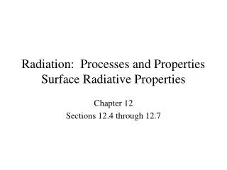
Net Radiation and Vegetation RN = Net radiation S = Downward shortwave (solar) radiation at the surface a = Net surface albedo (reflectivity) e = Emissivity L = Downward longwave (thermal) radiation from atmosphere s = Stefan Boltzmann constant TS = Surface temperature e 1 is usually a good assumption (blackbody assumption) a= 10% ‑ 40% (~80% over fresh snow) Sahara/Arabia 30‑35% Other deserts 20‑25% Dense forests 10‑15% (Compare to ocean 4‑5%) This summarizes the radiation balance at the land surface. Vegetation is particularly important in affecting the S term. Primary reference: Sellers, P. J., 1985: Canopy reflectance, photosynthesis and transpiration. Int. J. Remote Sensing, 6, 1335-1372. CLIM 714 Land-Climate Interactions
Biophysics • Photosynthesis • Plants use light (photsynthetically active radiation; PAR) as a source of energy to drive the chemical reaction that feeds the plant. • Photosynthesis combines water and carbon dioxide to produce sugar (basic fuel for all living organisms). • Plants produce oxygen as a biproduct of photosynthesis ‑ oxygen is waste to the plant. CLIM 714 Land-Climate Interactions
Biophysics • Transpiration • In the process of plant respiration (taking CO2 from the atmosphere through the stomata), plants lose water vapor • Plants are constantly trying to balance the benefit of gaining CO2 with the detriment of losing water • The water loss removes heat from the land surface (latent heating) This is the “other side” of the net radiation equation — the vegetation and soil play an important role in all of these terms. Photosynthesis particularly affects latent heat flux. CLIM 714 Land-Climate Interactions
The Plane-Parallel Simplification • Usually we assume that locally the earth is flat. • Radiation is divided into only two directions: UP and DOWN. • Each direction is a proxy for all radiation in that hemisphere (i.e., within each hemisphere of 2p steradians, radiant energy is isotropic) The plane is horizontal to the earth’s surface, and may represent any interface (between layers of the atmosphere, above and below a forest canopy, or even a single leaf in a vegetation canopy). CLIM 714 Land-Climate Interactions
Direct versus Diffuse Radiation • Shortwave radiation can be either direct (with a specific source in a specific direction), or diffuse (coming from all directions). • Direct radiation - (heliotropic) • Emanates from the sun, which is typically treated as a point source of radiation, traveling as a beam. • Can be absorbed, reflected, transmitted based on the specific location and geometry of clouds, mountains, leaves, buildings, etc. • Diffuse radiation - (isotropic) • Emanates from the entire hemisphere (above or below), and is scattered sunlight. e.g., the light coming from a clear blue sky (or a grey cloudy sky). • Has no specific direction, and is typically treated as uniform. • Thermal radiation (heat) is also typically treated as an isotropic diffuse radiation. CLIM 714 Land-Climate Interactions
Direct vs. Diffuse • In reality, diffuse radiation does vary across the sky, or the ground. And the sun is not a point source, but subtends a finite solid angle in the sky. For simplicity, the above assumptions are typically applied, and usually do not affect the net radiation balance by more than a few percent. A “fisheye” lens view of the sky (the upper hemisphere) at noon. Both clear sky and clouds contribute diffuse downward solar radiation. The disk on the right shows the idealization of the sky used in many radiative transfer calculations CLIM 714 Land-Climate Interactions
Direct Radiation in a Canopy Analogous to the transfer equation, we can describe extinction by a plant canopy: I = radiative flux, k = extinction coefficient, L = leaf area index. The extinction coefficient will depend on the orientation of the leaves: CLIM 714 Land-Climate Interactions
Direct Radiation in a Canopy Direct radiation comes from the direction of the solar zenith angle q so we can define an inverse optical depth: It interacts with the canopy depending on the orientation of the leaves. The projected area of the leaves can be represented as a function of the direction of radiation G(m), which may be quite complex depending on the shape and structure of the leaves and plants. The extinction coefficient is defined as: For a simple flat horizontal leaf, G(m) = m, so k = 1. CLIM 714 Land-Climate Interactions
Diffuse Radiation in a Canopy For diffuse radiation: And the scattering coefficient w = a + t is the sum of reflectance and transmittance. Most canopies have a fairly small scattering coefficient in the visible range (photosynthetically active radiation; PAR), and a very high scattering in the near infrared: PAR Region: w 0.2 NIR Region: w 0.95 CLIM 714 Land-Climate Interactions
Two-Stream Approximation • Assuming that the scattered (diffuse) fluxes are hemispherically integrated, we can split all of the fluxes of visible and near infrared radiation into 3 components: • Upward diffuse flux I • Downward diffuse flux I • Incident direct flux Io CLIM 714 Land-Climate Interactions
Two-Stream Formulation The equations for the change in diffuse flux as it penetrates the canopy (i.e. as a function of the LAI penetrated, where LAI is essentially a vertical coordinate within the canopy) are: b and bo are the upscatter parameter for diffuse and direct radiation respectively: is the mean leaf inclination angle relative to horizontal, andas(m)is the single scattering albedo. CLIM 714 Land-Climate Interactions
Two-Stream The pair of differential equations above can be solved given appropriate boundary conditions. Assuming a normalized incident solar radiation at the top of the canopy: and at the bottom where L = Ltotal: CLIM 714 Land-Climate Interactions
Leaf Area Index This is the fraction of the surface area covered by leaf surfaces when viewed from above. No leaves at all: LAI = 0. Imagine one giant leaf, covering everything like a blanket. The LAI would be 1. An actual canopy has multiple leaves overlying any point of the surface. The LAI can exceed 1. In fact, for very dense canopies, it may be 5, 6, 7, or more. The LAI over an area is the average number of horizontal surfaces intercepted while traveling down through the canopy to the top to the soil: CLIM 714 Land-Climate Interactions
Reflectance • In general: • In visible wavelengths, soil is dark, vegetation is darker. • In near-infrared wavelengths, soil is dark, canopy is bright. So LAI has a strong influence on the NIR albedo, but not so much on the visible albedo. The visible albedo is low, so that the fraction of photosynthetically active radiation absorbed by the plant (FPAR) is high. This optimizes the energy available for food production in the plant’s cells. CLIM 714 Land-Climate Interactions
Vegetation Indices This difference between albedos in PAR and NIR ranges allows us to define vegetation indices that can be used to estimate vegetation cover (and thus LAI) from remote sensing: Simple ratio: Normalized difference vegetation index: CLIM 714 Land-Climate Interactions
Canopy Photosynthesis APAR is the PAR absorbed by the green canopy. The fraction of PAR absorbed: where V stands for visible, and : CLIM 714 Land-Climate Interactions
Canopy Photosynthesis Meanwhile, the NIR is mostly reflected: Since aV is relatively constant with LAI for a canopy over dark soils: So vegetation index FPAR, and satellites may give us measurements of reflectance, photosynthesis, and transpiration. CLIM 714 Land-Climate Interactions
Friction Laminar Flow Laminar Flow Turbulent Flow Smooth, Frictionless (slip condition) Rough (no-slip condition) Earth’s surface is not smooth, frictionless, or inert. Thus there exist vertical wind speed, temperature, and moisture gradients. • Vertical gradients in wind are caused by the "no-slip" condition at the interface between the fluid (atmosphere) and solid surface: • Vertical gradients in temperature are caused by the different thermal and radiative properties of the surface and fluid. • Vertical gradients in moisture are caused by the different water holding properties of the surface and fluid. CLIM 714 Land-Climate Interactions
Surface Layers • How are energy, momentum and moisture exchanged in the boundary layer over the surface of the earth? • 0-10mm Molecular processes • 10mm-10m Frictional processes (constant stress layer) • 10m-2km Friction, pressure gradient, Coriolis (mixed layer) • The atmosphere “sees” the fluxes from the surface as lower boundary conditions, but flux divergence in the vertical determines how the surface fluxes affect the circulation and the thermal structure. As energy cascades to smaller scales, turbulence dissipates it. But turbulence can also transport energy across gradients — much more effectively than diffusion. This is key for energy fluxes between land and atmosphere. CLIM 714 Land-Climate Interactions
Land versus Ocean • Ocean has a much higher heat capacity than land. • Water “flows” while the land surface is fixed. Ocean can transport much heat laterally, land cannot. • Ocean, obviously, is wet (evaporation is not limited by lack of moisture). Land can be wet, dry, or somewhere in between (moisture limitations can impede evaporation). • The upper layer of the ocean is well mixed, so the surface characteristics are sufficient to define its interaction with the atmosphere, but soil has vertical structure and overlying vegetation. Heat conduction and moisture transport below the surface become important. • These facts have a bearing on the physical interactions between the surface and the atmosphere and on the manner in which drag coefficients are specified. CLIM 714 Land-Climate Interactions
The Planetary Boundary Layer (PBL) The PBL (shaded below) is the layer of the earth’s atmosphere between the earth’s surface and the free atmosphere (where the wind is essentially geostrophic); it includes the surface friction layer (constant stress layer) and the mixed layer (Ekman layer). Over land, the PBL height varies from 0 to 2000m with a strong diurnal cycle. Over ocean, it is typically 100—700m thick. CLIM 714 Land-Climate Interactions
Constant Stress Layer Mixed Layer z~0.1h V Θ q τ Ho Eo Constant Stress Layer Vo Θo qo zo (Ts, qs) LAND (Ts, Vs) OCEAN This layer near the surface is of primary concern for land-atmosphere interactions; it lies between the soil/vegetation models and the AGCM. z = top of the constant stress layer zo = roughness length, h = depth of PBL V = Wind velocity Q = Potential temperature q = Specific humidity Note: Vo = 0 over land (assumed), Vo = Vs over ocean CLIM 714 Land-Climate Interactions
Turbulent Fluxes Vertical fluxes of momentum, latent heat and sensible heat can be written as: where the turbulent stress (the second order terms in each) is related to the flux gradient in the vertical. For example, for momentum, t is the tangential frictional force. The shear normal to the surface is: Turbulence closure schemes like those applied in the Ekman layer are built around the expansion of the higher order terms to some level after which derivatives of the higher order moments → 0. CLIM 714 Land-Climate Interactions
Turbulent Fluxes The far RHS terms are applied in the "Mixing Length" method (also known as "K theory"). KM, KH, and KW are the eddy viscosity, eddy thermal diffusivity and eddy diffusivity for moisture respectively. They represent the efficiency with which mixing (i.e., vertical fluxes) occurs for a given shear, and are a property of the fluid under consideration. Turbulent mixing occurs over a length scale l that is a function of the depth of the constant stress layer: k is the von Karman constant (0.4 as determined experimentally). CLIM 714 Land-Climate Interactions
Monin-Obukhov Similarity Theory Near an interface (e.g., the surface of the earth) we must be concerned with the effects of the discontinuities in temperature and moisture, and the effect of the "no-slip" boundary condition on turbulent transfer. We can relate the viscosity to the length scale through a frictional velocity: The frictional velocity is a function of the horizontal surface stress: Disregarding the direction of the wind, and substituting we have: CLIM 714 Land-Climate Interactions
Monin-Obukhov Similarity Theory Integrating in z: The constant of integration is chosen asC = ln(zo) such thatu = 0 atz = zo. zois called the roughness length. So: zo1—10 cm over a smooth surface like bare ground 1—10 m over a varied canopy of tall trees. Note: typically z is not measured from the ground, but from a reference level called the displacement height d which is the level of action of surface drag. CLIM 714 Land-Climate Interactions
Displacement Height and Drag Note: typically z is not measured from the ground, but from a reference level called the displacement height d which is the level of action of surface drag. This may be far aloft in the canopy where vegetation is present. This is done to ensure a good fit to the logarithmic relationship: Where Z is the actual height above the ground. Where Z>>d, the displacement height can be ignored. In bulk transfer relationships we can define a drag coefficient: Note: This is for “neutral” conditions (i.e. the vertical lapse rate of temperature is such that in the absence of diffusion, a parcel displaced vertically would heat/cool adiabatically to the temperature at its new elevation). In non-neutral conditions, this gets more complicated! CLIM 714 Land-Climate Interactions
Drag Coefficients Similar drag coefficients can be defined for heat and moisture (often chosen to be the same) based on a surface scaling length for heat that yields a zH analogous to zo: So by analogy we can define the bulk transfer relations in terms of drag coefficients: Here u is a non-directional wind speed, and likewise the momentum flux to is non-directional. CLIM 714 Land-Climate Interactions
Aerodynamic Resistance Finally, if we recognize that (CD u) and its brethren are conductances that facilitate the rate of flux, given a certain gradient, then we may define aerodynamic resistances: So that: This final formulation is typically used in Land Surface Schemes (LSS), and is the basis of turbulent fluxes within the Simple Biosphere (SiB) model and its so-called SiBlings. Primary reference: Garratt, J. R., 1992: The atmospheric boundary layer. Cambridge University Press, 316 pp. CLIM 714 Land-Climate Interactions