Download
1 / 36
360 likes | 726 Views
Metropolis light transport. Digital Image Synthesis Yung-Yu Chuang 12/27/2007. with slides by Matt Pharr . Metropolis sampling. Another way to generate samples from a distribution (similar to inversion, rejection and transform) Problem: given an arbitrary function assuming

E N D
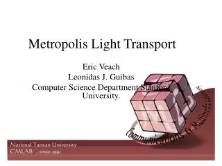
Metropolis light transport Digital Image Synthesis Yung-Yu Chuang 12/27/2007 with slides by Matt Pharr
Metropolis sampling • Another way to generate samples from a distribution (similar to inversion, rejection and transform) • Problem: given an arbitrary function assuming generate a set of samples
Metropolis sampling • MS only requires the ability to evaluate f without requiring integrating f, normalizing f nor inversion. • Steps • Generate initial sample x0 • mutating current sample xi to propose x’ • If it is accepted, xi+1 = x’ Otherwise, xi+1 = xi • Acceptance probability guarantees distribution is the stationary distribution f
Metropolis sampling • Mutations propose x’ given xi • T(x→x’) is the tentative transition probability density of proposing x’ from x • Being able tocalculate tentative transition probability is the only restriction for the choice of mutations • a(x→x’) is the acceptance probability of accepting the transition • By defining a(x→x’) carefully, we ensure
Metropolis sampling • Detailed balance stationary distribution
Acceptance probability • Does not affect unbiasedness; just variance • Want transitions to happen because transitions are often heading where f is large • Maximize the acceptance probability • Explore state space better • Reduce correlation
Mutation strategy • Very free and flexible, only need to calculate transition probability • Based on applications and experience • The more mutation, the better • Relative frequency of them is not so important
1D example mutation 1 mutation 2 10,000 iterations
1D example mutation 1 mutation 2 300,000 iterations
1D example mutation 1 90% mutation 2 + 10% mutation 1 Periodically using uniform mutations increases ergodicity
2D example (image copy) 1 sample per pixel 8 samples per pixel 256 samples per pixel
Results Distributed ray tracing Metropolis sampling
Metropolis light transport • Veach and Guibas introduced Metropolis sampling to Graphics from computational physics in their SIGGRAPH 1997 paper, Metropolis Light Transport. • Unbiased and robust (can deal with difficult cases such as caustics) • However, difficult to understand and implement efficiently. • Few implementation exists such as Indigo renderer and Kerkythea.
Metropolis light transport • Each path is generated by mutating previous path. • Advantages: • Path reuse: efficient • Local exploration: explore important contributions, reducing variance
Lens perturbation and pixel stratification • Make sure every pixel is covered somehow.
Results Bidirectional Path tracing 25 samples per pixel
Results Metropolis light transport With the same number of ray queries
Results Bidirectional path tracing (40 samples per pixel)
Results Metropolis light transport (average 250 mutations per pixel, same computation time as the above)