Download
1 / 43
430 likes | 565 Views
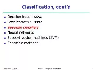
Classification, cont’d. Decision trees : done Lazy learners : done Bayesian classifiers Neural networks Support-vector machines (SVM) Ensemble methods. Bayesian Classification: Why?.

E N D
Classification, cont’d • Decision trees : done • Lazy learners : done • Bayesian classifiers • Neural networks • Support-vector machines (SVM) • Ensemble methods Machine Leaning: An Introduction
Bayesian Classification: Why? • A statistical classifier: performs probabilistic prediction, i.e., predicts class membership probabilities • Foundation: Based on Bayes’ Theorem. • Performance: A simple Bayesian classifier, naïve Bayesian classifier, has comparable performance with decision tree and selected neural network classifiers • Incremental: Each training example can incrementally increase/decrease the probability that a hypothesis is correct • Standard: Even when Bayesian methods are computationally intractable, they can provide a standard of optimal decision making against which other methods can be measured Machine Leaning: An Introduction
Bayesian Theorem: Basics • Let X be a data sample and C a class • P(C|X) : Proba that X belongs to class C given the attribute description of X • Given classes C1, C2 … Cm , we should assign X to the class Ci s.t. P(Ci|X) is maximum • We can assess P(Ci|X) using Bayes’ rule: Machine Leaning: An Introduction
Bayesian Theorem (cont’d) • P(C): Proba that X belongs to class C independently of the attributes of X • P(X): Proba that sample data is observed • P(X|C): Proba of observing the sample X, knowing it belongs to class C • Practical difficulty: require initial knowledge of many probabilities, significant computational cost Machine Leaning: An Introduction
An example Machine Leaning: An Introduction
Towards Naïve Bayesian Classifier • Let D be a training set of tuples and their associated class labels, and each tuple is represented by an n-D attribute vector X = (x1, x2, …, xn) • Suppose there are m classes C1, C2, …, Cm. • Classification should maximise P(Ci|X) • This can be derived from Bayes’ theorem • Since P(X) is constant for all classes, only needs to be maximized Machine Leaning: An Introduction
Derivation of Naïve Bayes Classifier • A simplified assumption: attributes are conditionally independent (i.e., no dependence relation between attributes): • This greatly reduces the computation cost: Only counts the class distribution • If Ak is categorical, P(xk|Ci) is the # of tuples in Ci having value xk for Ak divided by |Ci, D| (# of tuples of Ci in D) • If Ak is continous-valued, P(xk|Ci) is usually computed based on Gaussian distribution with a mean μ and standard deviation σ and P(xk|Ci) is Machine Leaning: An Introduction
Naïve Bayesian Classifier: Training Dataset Class: C1:buys_computer = ‘yes’ C2:buys_computer = ‘no’ Data sample X = (age <=30, Income = medium, Student = yes Credit_rating = Fair) Machine Leaning: An Introduction
Naïve Bayesian Classifier: An Example • P(Ci): P(buys_computer = “yes”) = 9/14 = 0.643 P(buys_computer = “no”) = 5/14= 0.357 • Compute P(X|Ci) for each class P(age = “<=30” | buys_computer = “yes”) = 2/9 = 0.222 P(age = “<= 30” | buys_computer = “no”) = 3/5 = 0.6 P(income = “medium” | buys_computer = “yes”) = 4/9 = 0.444 P(income = “medium” | buys_computer = “no”) = 2/5 = 0.4 P(student = “yes” | buys_computer = “yes) = 6/9 = 0.667 P(student = “yes” | buys_computer = “no”) = 1/5 = 0.2 P(credit_rating = “fair” | buys_computer = “yes”) = 6/9 = 0.667 P(credit_rating = “fair” | buys_computer = “no”) = 2/5 = 0.4 • X = (age <= 30 , income = medium, student = yes, credit_rating = fair) P(X|Ci) : P(X|buys_computer = “yes”) = 0.222 x 0.444 x 0.667 x 0.667 = 0.044 P(X|buys_computer = “no”) = 0.6 x 0.4 x 0.2 x 0.4 = 0.019 P(X|Ci)*P(Ci) : P(X|buys_computer = “yes”) * P(buys_computer = “yes”) = 0.028 P(X|buys_computer = “no”) * P(buys_computer = “no”) = 0.007 Therefore, X belongs to class (“buys_computer = yes”) Machine Leaning: An Introduction
Avoiding the 0-Probability Problem • Naïve Bayesian prediction requires each conditional prob. be non-zero. Otherwise, the predicted prob. will be zero • Eg., suppose a dataset with 1000 tuples, income can be low (0 example), medium (990 ex.) or high (10 ex.), • Use Laplacian correction (or Laplacian estimator) • Adding 1 to each case Prob(income = low) = 1/1003 Prob(income = medium) = 991/1003 Prob(income = high) = 11/1003 • The “corrected” prob. estimates are close to their “uncorrected” counterparts Machine Leaning: An Introduction
Naïve Bayesian Classifier: Comments • Advantages • Easy to implement • Good results obtained in most of the cases • Disadvantages • Assumption: class conditional independence, therefore loss of accuracy • Practically, dependencies exist among variables • E.g., hospitals: patients: Profile: age, family history, etc. Symptoms: fever, cough etc., Disease: lung cancer, diabetes, etc. • Dependencies among these cannot be modeled by Naïve Bayesian Classifier • How to deal with these dependencies? • Bayesian Belief Networks Machine Leaning: An Introduction
Y Z P Bayesian Belief Networks • Bayesian belief network allows a subset of the variables conditionally independent • A graphical model of causal relationships • Represents dependency among the variables • Gives a specification of joint probability distribution • Nodes: random variables • Links: dependency • X and Y are the parents of Z, and Y is the parent of P • No dependency between Z and P • Has no loops or cycles X Machine Leaning: An Introduction
(FH, S) (FH, ~S) (~FH, S) (~FH, ~S) LC 0.8 0.7 0.5 0.1 ~LC 0.2 0.5 0.3 0.9 Bayesian Belief Network: An Example Family History Smoker The conditional probability table (CPT) for variable LungCancer: LungCancer Emphysema CPT shows the conditional probability for each possible combination of its parents PositiveXRay Dyspnea Derivation of the probability of a particular combination of values of X, from CPT: Bayesian Belief Networks Machine Leaning: An Introduction
Training Bayesian Networks Several scenarios: • Given both the network structure and all variables observable: learn only the CPTs • Network structure known, some hidden variables: gradient descent (greedy hill-climbing) method, analogous to neural network learning • Network structure unknown, all variables observable: search through the model space to reconstruct network topology • Unknown structure, some hidden variables: No good algorithm known yet for this purpose Machine Leaning: An Introduction
Classification cont’d • Decision trees • Lazy learners • Bayesian classifiers • Neural networks • Support-vector machines (SVM) • Ensemble methods Machine Leaning: An Introduction
Classification by Backpropagation • Backpropagation: A neural network learning algorithm • Started by psychologists and neurobiologists to develop and test computational analogues of neurons • A neural network: A set of connected input/output units where each connection has a weight associated with it • During the learning phase, the network learns by adjusting the weights so as to be able to predict the correct class label of the input tuples • Also referred to as connectionist learning due to the connections between units Machine Leaning: An Introduction
Neural Network as a Classifier • Weakness • Long training time • Require a number of parameters typically best determined empirically, e.g., the network topology or ``structure." • Poor interpretability: Difficult to interpret the symbolic meaning behind the learned weights and of ``hidden units" in the network • Strength • High tolerance to noisy data • Ability to classify untrained patterns • Well-suited for continuous-valued inputs and outputs • Successful on a wide array of real-world data • Algorithms are inherently parallel • Techniques have recently been developed for the extraction of rules from trained neural networks Machine Leaning: An Introduction
- mk x0 w0 x1 w1 f å output y xn wn Input vector x weight vector w weighted sum Activation function A Neuron (= a perceptron) • The n-dimensional input vector x is mapped into variable y by means of the scalar product and a nonlinear function mapping Machine Leaning: An Introduction
A Multi-Layer Feed-Forward Neural Network Output vector Output layer Hidden layer wij Input layer Input vector: X Machine Leaning: An Introduction
How A Multi-Layer Neural Network Works? • The inputs to the network correspond to the attributes measured for each training tuple • Inputs are fed simultaneously into the units making up the input layer • They are then weighted and fed simultaneously to a hidden layer • The number of hidden layers is arbitrary, although usually only one • The weighted outputs of the last hidden layer are input to units making up the output layer, which emits the network's prediction • The network is feed-forward in that none of the weights cycles back to an input unit or to an output unit of a previous layer • From a statistical point of view, networks perform nonlinear regression: Given enough hidden units and enough training samples, they can closely approximate any function Machine Leaning: An Introduction
Defining a Network Topology • First decide the network topology: # of units in the input layer, # of hidden layers (if > 1), # of units in each hidden layer, and # of units in the output layer • Normalizing the input values for each attribute measured in the training tuples to [0.0—1.0] • One input unit per domain value, each initialized to 0 • Output, if for classification and more than two classes, one output unit per class is used • Once a network has been trained and its accuracy is unacceptable, repeat the training process with a different network topology or a different set of initial weights Machine Leaning: An Introduction
Backpropagation • Iteratively process a set of training tuples & compare the network's prediction with the actual known target value • For each training tuple, the weights are modified to minimize the mean squared error between the network's prediction and the actual target value • Modifications are made in the “backwards” direction: from the output layer, through each hidden layer down to the first hidden layer, hence “backpropagation” • Steps • Initialize weights (to small random #s) and biases in the network • Propagate the inputs forward (by applying activation function) • Backpropagate the error (by updating weights and biases) • Terminating condition (when error is very small, etc.) Machine Leaning: An Introduction
A Multi-Layer Feed-Forward Neural Network Output vector Output layer Hidden layer wij Input layer Input vector: X Machine Leaning: An Introduction
Backpropagation and Interpretability • Efficiency of backpropagation: Each epoch (one iteration through the training set) takes O(|D| * w), with |D| tuples and w weights, but # of epochs can be exponential to n, the number of inputs, in the worst case • Rule extraction from networks: network pruning • Simplify the network structure by removing weighted links that have the least effect on the trained network • Then perform link, unit, or activation value clustering • The set of input and activation values are studied to derive rules describing the relationship between the input and hidden unit layers • Sensitivity analysis: assess the impact that a given input variable has on a network output. The knowledge gained from this analysis can be represented in rules Machine Leaning: An Introduction
Classification cont’d • Decision trees • Lazy learners • Bayesian classifiers • Neural networks • Support-vector machines (SVM) • Ensemble methods Machine Leaning: An Introduction
SVM—Support Vector Machines • A classification method for both linear and nonlinear data • It uses a nonlinear mapping to transform the original training data into a higher dimension • With the new dimension, it searches for the linear optimal separating hyperplane (i.e., “decision boundary”) • With an appropriate nonlinear mapping to a sufficiently high dimension, data from two classes can always be separated by a hyperplane • SVM finds this hyperplane using support vectors (“essential” training tuples) and margins (defined by the support vectors) Machine Leaning: An Introduction
SVM—History and Applications • Vapnik and colleagues (1992)—groundwork from Vapnik & Chervonenkis’ statistical learning theory in 1960s • Features: training can be slow but accuracy is high owing to their ability to model complex nonlinear decision boundaries (margin maximization) • Used both for classification and prediction, including structured outputs (e.g. graphs) Machine Leaning: An Introduction
Small Margin Large Margin Support Vectors SVM—General Philosophy Machine Leaning: An Introduction
SVM—When Data Is Linearly Separable m Let data D be (X1, y1), …, (X|D|, y|D|), where Xi is the set of training tuples associated with the class labels yi There are infinite lines (hyperplanes) separating the two classes but we want to find the best one (the one that minimizes classification error on unseen data) SVM searches for the hyperplane with the largest margin, i.e., maximum marginal hyperplane (MMH) Machine Leaning: An Introduction
SVM—Linearly Separable • A separating hyperplane can be written as W ● X + b = 0 where W={w1, w2, …, wn} is a weight vector and b a scalar (bias) • For 2-D it can be written as w0 + w1 x1 + w2 x2 = 0 • The hyperplane defining the sides of the margin: H1: w0 + w1 x1 + w2 x2 ≥ 1 for yi = +1, and H2: w0 + w1 x1 + w2 x2 ≤ – 1 for yi = –1 • Any training tuples that fall on hyperplanes H1 or H2 (i.e., the sides defining the margin) are support vectors • This becomes a constrained (convex) quadratic optimization problem: Quadratic objective function and linear constraints Quadratic Programming (QP) Lagrangian multipliers Machine Leaning: An Introduction
Why Is SVM Effective on High Dimensional Data? • The complexity of trained classifier is characterized by the # of support vectors rather than the dimensionality of the data • The support vectors are the essential or critical training examples —they lie closest to the decision boundary (MMH) • If all other training examples are removed and the training is repeated, the same separating hyperplane would be found • The number of support vectors found can be used to compute an (upper) bound on the expected error rate of the SVM classifier, which is independent of the data dimensionality • Thus, an SVM with a small number of support vectors can have good generalization, even when the dimensionality of the data is high Machine Leaning: An Introduction
SVM—Linearly Inseparable • Transform the original input data into a higher dimensional space • Search for a linear separating hyperplane in the new space Machine Leaning: An Introduction
SVM—Kernel functions • Instead of computing the dot product on the transformed data tuples, it is mathematically equivalent to instead applying a kernel function K(Xi, Xj) to the original data, i.e., K(Xi, Xj) = Φ(Xi) Φ(Xj) • Typical Kernel Functions • SVM can also be used for classifying multiple (> 2) classes and for regression analysis (with additional user parameters) Machine Leaning: An Introduction
SVM Relatively new concept Deterministic algorithm Nice Generalization properties Hard to learn – learned in batch mode using quadratic programming techniques Using kernels can learn very complex functions Neural Network Relatively old Nondeterministic algorithm Generalizes well but doesn’t have strong mathematical foundation Can easily be learned in incremental fashion To learn complex functions—use multilayer perceptron (not that trivial) SVM vs. Neural Network Machine Leaning: An Introduction
Classification cont’d • Decision trees • Lazy learners • Bayesian classifiers • Neural networks • Support-vector machines (SVM) • Ensemble methods Machine Leaning: An Introduction
Ensemble Methods: Increasing the Accuracy • Ensemble methods • Use a combination of models to increase accuracy • Combine a series of k learned models, M1, M2, …, Mk, with the aim of creating an improved model M* • Popular ensemble methods • Bagging: averaging the prediction over a collection of classifiers • Boosting: weighted vote with a collection of classifiers • Ensemble: combining a set of heterogeneous classifiers Machine Leaning: An Introduction
Bagging: Boostrap Aggregation • Analogy: Diagnosis based on multiple doctors’ majority vote • Training • Given a set D of d tuples, at each iteration i, a training set Di of d tuples is sampled with replacement from D (i.e., boostrap) • A classifier model Mi is learned for each training set Di • Classification: classify an unknown sample X • Each classifier Mi returns its class prediction • The bagged classifier M* counts the votes and assigns the class with the most votes to X • Prediction: can be applied to the prediction of continuous values by taking the average value of each prediction for a given test tuple • Accuracy • Often significant better than a single classifier derived from D • For noisy data: not considerably worse, more robust • Proved improved accuracy in prediction Machine Leaning: An Introduction
Boosting • Analogy: Consult several doctors, based on a combination of weighted diagnoses—weight assigned based on the previous diagnosis accuracy • How boosting works? • Weights are assigned to each training tuple • A series of k classifiers is iteratively learned • After a classifier Mi is learned, the weights are updated to allow the subsequent classifier, Mi+1, to pay more attention to the training tuples that were misclassified by Mi • The final M* combines the votes of each individual classifier, where the weight of each classifier's vote is a function of its accuracy • The boosting algorithm can be extended for the prediction of continuous values • Comparing with bagging: boosting tends to achieve greater accuracy, but it also risks overfitting the model to misclassified data Machine Leaning: An Introduction
Adaboost (Freund and Schapire, 1997) • Given a set of d class-labeled tuples, (X1, y1), …, (Xd, yd) • Initially, all the weights of tuples are set the same (1/d) • Generate k classifiers in k rounds. At round i, • Tuples from D are sampled (with replacement) to form a training set Di of the same size • Each tuple’s chance of being selected is based on its weight • A classification model Mi is derived from Di • Its error rate is calculated using Di as a test set • If a tuple is misclassified, its weight is increased, else it is decreased • Error rate: err(Xj) is the misclassification error of tuple Xj. Classifier Mi error rate is the sum of the weights of the misclassified tuples: • The weight of classifier Mi’s vote is Machine Leaning: An Introduction
References (1) • C. Apte and S. Weiss. Data mining with decision trees and decision rules. Future Generation Computer Systems, 13, 1997. • C. M. Bishop, Neural Networks for Pattern Recognition. Oxford University Press, 1995. • L. Breiman, J. Friedman, R. Olshen, and C. Stone. Classification and Regression Trees. Wadsworth International Group, 1984. • C. J. C. Burges. A Tutorial on Support Vector Machines for Pattern Recognition. Data Mining and Knowledge Discovery, 2(2): 121-168, 1998. • P. K. Chan and S. J. Stolfo. Learning arbiter and combiner trees from partitioned data for scaling machine learning. KDD'95. • W. Cohen. Fast effective rule induction. ICML'95. • G. Cong, K.-L. Tan, A. K. H. Tung, and X. Xu. Mining top-k covering rule groups for gene expression data. SIGMOD'05. • A. J. Dobson. An Introduction to Generalized Linear Models. Chapman and Hall, 1990. • G. Dong and J. Li. Efficient mining of emerging patterns: Discovering trends and differences. KDD'99. Machine Leaning: An Introduction
References (2) • R. O. Duda, P. E. Hart, and D. G. Stork. Pattern Classification, 2ed. John Wiley and Sons, 2001 • U. M. Fayyad. Branching on attribute values in decision tree generation. AAAI’94. • Y. Freund and R. E. Schapire. A decision-theoretic generalization of on-line learning and an application to boosting. J. Computer and System Sciences, 1997. • J. Gehrke, R. Ramakrishnan, and V. Ganti. Rainforest: A framework for fast decision tree construction of large datasets. VLDB’98. • J. Gehrke, V. Gant, R. Ramakrishnan, and W.-Y. Loh, BOAT -- Optimistic Decision Tree Construction. SIGMOD'99. • T. Hastie, R. Tibshirani, and J. Friedman. The Elements of Statistical Learning: Data Mining, Inference, and Prediction. Springer-Verlag, 2001. • D. Heckerman, D. Geiger, and D. M. Chickering. Learning Bayesian networks: The combination of knowledge and statistical data. Machine Learning, 1995. • M. Kamber, L. Winstone, W. Gong, S. Cheng, and J. Han. Generalization and decision tree induction: Efficient classification in data mining. RIDE'97. • B. Liu, W. Hsu, and Y. Ma. Integrating Classification and Association Rule. KDD'98. • W. Li, J. Han, and J. Pei, CMAR: Accurate and Efficient Classification Based on Multiple Class-Association Rules, ICDM'01. Machine Leaning: An Introduction
References (3) • T.-S. Lim, W.-Y. Loh, and Y.-S. Shih. A comparison of prediction accuracy, complexity, and training time of thirty-three old and new classification algorithms. Machine Learning, 2000. • J. Magidson. The Chaid approach to segmentation modeling: Chi-squared automatic interaction detection. In R. P. Bagozzi, editor, Advanced Methods of Marketing Research, Blackwell Business, 1994. • M. Mehta, R. Agrawal, and J. Rissanen. SLIQ : A fast scalable classifier for data mining. EDBT'96. • T. M. Mitchell. Machine Learning. McGraw Hill, 1997. • S. K. Murthy, Automatic Construction of Decision Trees from Data: A Multi-Disciplinary Survey, Data Mining and Knowledge Discovery 2(4): 345-389, 1998 • J. R. Quinlan. Induction of decision trees. Machine Learning, 1:81-106, 1986. • J. R. Quinlan and R. M. Cameron-Jones. FOIL: A midterm report. ECML’93. • J. R. Quinlan. C4.5: Programs for Machine Learning. Morgan Kaufmann, 1993. • J. R. Quinlan. Bagging, boosting, and c4.5. AAAI'96. Machine Leaning: An Introduction
References (4) • R. Rastogi and K. Shim. Public: A decision tree classifier that integrates building and pruning. VLDB’98. • J. Shafer, R. Agrawal, and M. Mehta. SPRINT : A scalable parallel classifier for data mining. VLDB’96. • J. W. Shavlik and T. G. Dietterich. Readings in Machine Learning. Morgan Kaufmann, 1990. • P. Tan, M. Steinbach, and V. Kumar. Introduction to Data Mining. Addison Wesley, 2005. • S. M. Weiss and C. A. Kulikowski. Computer Systems that Learn: Classification and Prediction Methods from Statistics, Neural Nets, Machine Learning, and Expert Systems. Morgan Kaufman, 1991. • S. M. Weiss and N. Indurkhya. Predictive Data Mining. Morgan Kaufmann, 1997. • I. H. Witten and E. Frank. Data Mining: Practical Machine Learning Tools and Techniques, 2ed. Morgan Kaufmann, 2005. • X. Yin and J. Han. CPAR: Classification based on predictive association rules. SDM'03 • H. Yu, J. Yang, and J. Han. Classifying large data sets using SVM with hierarchical clusters. KDD'03. Machine Leaning: An Introduction