Pairwise Alignments

1. Pairwise Alignments Biology 224 Instructor: Tom Peavy Sept 14 &16 <PowerPoint slides based on Bioinformatics and Functional Genomics by Jonathan Pevsner>

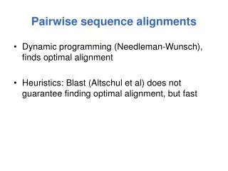
2. General approach to pairwise alignment • Choose two sequences • Select an algorithm that generates a score • Allow gaps (insertions, deletions) • Score reflects degree of similarity • Alignments can be global or local • Estimate probability that the alignment • occurred by chance

3. “Scoring matrices” let us assign scores for each aligned amino acid in a pairwise alignment. What should the score be when a serine matches a serine, or a threonine, or a valine? Can we devise “lenient” scoring systems to help us align distantly related proteins, and more conservative scoring systems to align closely related proteins?

4. Calculation of an alignment score http://www.ncbi.nlm.nih.gov/Education/BLASTinfo/Alignment_Scores2.html

5. Scoring Matrices take into account: Conservation – acceptable substitutions while not changing function of protein (charge, size, hydrophobicity) Frequency – reflect how often particular residues occur among entire collection of proteins (rare residues given more weight) Evolution – different scoring matrices are designed to either detect closely related or more distantly related proteins

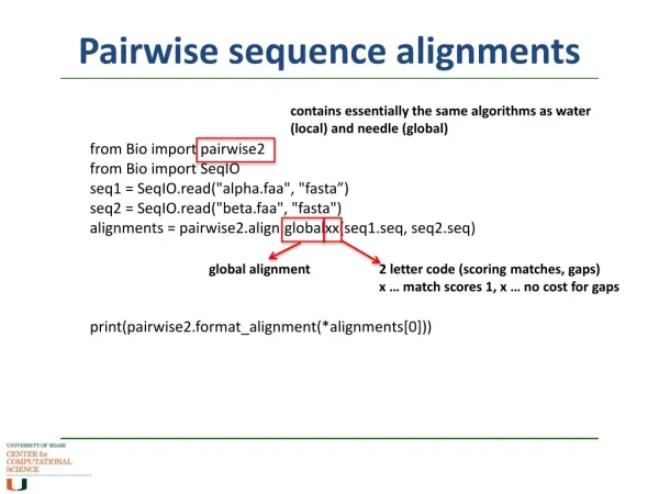
6. Two kinds of sequence alignment: global and local global alignment algorithm --Needleman and Wunsch (1970) local alignment algorithm --Smith and Waterman (1981)

7. Global alignment versus local alignment Global alignment (Needleman-Wunsch) extends from one end of each sequence to the other Local alignment finds optimally matching regions within two sequences (“subsequences”) Local alignment is almost always used for database searches such as BLAST. It is useful to find domains (or limited regions of homology) within sequences Smith and Waterman (1981) solved the problem of performing optimal local sequence alignment. Other methods (BLAST, FASTA) are faster but less thorough.

8. Global alignment with the algorithm of Needleman and Wunsch (1970) • • Two sequences can be compared in a matrix • along x- and y-axes. • • If they are identical, a path along a diagonal • can be drawn • • Find the optimal subpaths, and add them up to achieve • the best score. This involves • --adding gaps when needed • --allowing for conservative substitutions • --choosing a scoring system (simple or complicated) • N-W is guaranteed to find optimal alignment(s)

9. Three steps to global alignment with the Needleman-Wunsch algorithm [1] set up a matrix [2] score the matrix [3] identify the optimal alignment(s)

10. Four possible outcomes in aligning two sequences 1 2 [1] identity (stay along a diagonal) [2] mismatch (stay along a diagonal) [3] gap in one sequence (move vertically!) [4] gap in the other sequence (move horizontally!)

11. Try using needle to implement a Needleman-Wunsch global alignment algorithm to find the optimum alignment (including gaps): http://www.ebi.ac.uk/emboss/align/

12. Queries: beta globin (NP_000509) alpha globin (NP_000549)

13. Local Alignment How the Smith-Waterman algorithm works Set up a matrix between two proteins (size m+1, n+1) No values in the scoring matrix can be negative! S > 0 The score in each cell is the maximum of four values: [1] s(i-1, j-1) + the new score at [i,j] (a match or mismatch) [2] s(i,j-1) – gap penalty [3] s(i-1,j) – gap penalty [4] zero

14. Smith-Waterman local alignment algorithm

15. Rapid, heuristic versions of Smith-Waterman: FASTA and BLAST Smith-Waterman is very rigorous and it is guaranteed to find an optimal alignment. But Smith-Waterman is slow. It requires computer space and time proportional to the product of the two sequences being aligned (or the product of a query against an entire database). Gotoh (1982) and Myers and Miller (1988) improved the algorithms so both global and local alignment require less time and space. FASTA and BLAST provide rapid alternatives to S-W

16. Try using SSEARCH to perform a rigorous Smith-Waterman local alignment: http://fasta.bioch.virginia.edu/

17. Queries: beta globin (NP_000509) alpha globin (NP_000549)

18. How FASTA works [1] A “lookup table” is created. It consists of short stretches of amino acids (e.g. k=3 for a protein search). The length of a stretch is called a k-tuple. The FASTA algorithm finds the ten highest scoring segments that align to the query. [2] These ten aligned regions are re-scored with a PAM or BLOSUM matrix. [3] High-scoring segments are joined. [4] Needleman-Wunsch or Smith-Waterman is then performed.

19. Pairwise alignment: BLAST 2 sequences • Go to http://www.ncbi.nlm.nih.gov/BLAST • Choose BLAST 2 sequences • In the program, [1] choose blastp or blastn [2] paste in your accession numbers (or use FASTA format) [3] select optional parameters --3 BLOSUM and 3 PAM matrices --gap creation and extension penalties --filtering --word size [4] click “align”

20. Page 73

21. Page 74

22. Statistical significance of pairwise alignment We will discuss the statistical significance of alignment scores in the BLAST lectures. A basic question is how to determine whether a particular alignment score is likely to have occurred by chance. According to the null hypothesis, two aligned sequences are not homologous (evolutionarily related). Can we reject the null hypothesis at a particular significance level alpha?

23. homologous sequences non-homologous sequences Sequences reported as related True positives False positives Sequences reported as unrelated False negatives True negatives Sensitivity: ability to find true positives Specificity: ability to minimize false positives

24. Substitution Matrix A substitution matrix contains values proportional to the probability that amino acid i mutates into amino acid j for all pairs of amino acids. Substitution matrices are constructed by assembling a large and diverse sample of verified pairwise alignments (or multiple sequence alignments) of amino acids. Substitution matrices should reflect the true probabilities of mutations occurring through a period of evolution. The two major types of substitution matrices are PAM and BLOSUM.

25. Dayhoff et al. examined multiple sequence alignments (e.g. glyceraldehyde 3-phosphate dehydrogenases) to generate tables of accepted point mutations fly GAKKVIISAP SAD.APM..F VCGVNLDAYK PDMKVVSNAS CTTNCLAPLA human GAKRVIISAP SAD.APM..F VMGVNHEKYD NSLKIISNAS CTTNCLAPLA plant GAKKVIISAP SAD.APM..F VVGVNEHTYQ PNMDIVSNAS CTTNCLAPLA bacterium GAKKVVMTGP SKDNTPM..F VKGANFDKY. AGQDIVSNAS CTTNCLAPLA yeast GAKKVVITAP SS.TAPM..F VMGVNEEKYT SDLKIVSNAS CTTNCLAPLA archaeon GADKVLISAP PKGDEPVKQL VYGVNHDEYD GE.DVVSNAS CTTNSITPVA fly KVINDNFEIV EGLMTTVHAT TATQKTVDGP SGKLWRDGRG AAQNIIPAST human KVIHDNFGIV EGLMTTVHAI TATQKTVDGP SGKLWRDGRG ALQNIIPAST plant KVVHEEFGIL EGLMTTVHAT TATQKTVDGP SMKDWRGGRG ASQNIIPSST bacterium KVINDNFGII EGLMTTVHAT TATQKTVDGP SHKDWRGGRG ASQNIIPSST yeast KVINDAFGIE EGLMTTVHSL TATQKTVDGP SHKDWRGGRT ASGNIIPSST archaeon KVLDEEFGIN AGQLTTVHAY TGSQNLMDGP NGKP.RRRRA AAENIIPTST fly GAAKAVGKVI PALNGKLTGM AFRVPTPNVS VVDLTVRLGK GASYDEIKAK human GAAKAVGKVI PELNGKLTGM AFRVPTANVS VVDLTCRLEK PAKYDDIKKV plant GAAKAVGKVL PELNGKLTGM AFRVPTSNVS VVDLTCRLEK GASYEDVKAA bacterium GAAKAVGKVL PELNGKLTGM AFRVPTPNVS VVDLTVRLEK AATYEQIKAA yeast GAAKAVGKVL PELQGKLTGM AFRVPTVDVS VVDLTVKLNK ETTYDEIKKV archaeon GAAQAATEVL PELEGKLDGM AIRVPVPNGS ITEFVVDLDD DVTESDVNAA Examined 1572 changes in 71 groups of closely related proteins

26. lys found at 58% of arg sites Emile Zuckerkandl and Linus Pauling (1965) considered substitution frequencies in 18 globins (myoglobins and hemoglobins from human to lamprey). Black: identity Gray: very conservative substitutions (>40% occurrence) White: fairly conservative substitutions (>21% occurrence) Red: no substitutions observed Page 80

27. Dayhoff’s 34 protein superfamilies ProteinPAMs per 100 million years Ig kappa chain 37 Kappa casein 33 luteinizing hormone b 30 lactalbumin 27 complement component 3 27 epidermal growth factor 26 proopiomelanocortin 21 pancreatic ribonuclease 21 haptoglobin alpha 20 serum albumin 19 phospholipase A2, group IB 19 prolactin 17 carbonic anhydrase C 16 Hemoglobin a 12 Hemoglobin b 12

28. Dayhoff’s 34 protein superfamilies ProteinPAMs per 100 million years Ig kappa chain 37 Kappa casein 33 luteinizing hormone b 30 lactalbumin 27 complement component 3 27 epidermal growth factor 26 proopiomelanocortin 21 pancreatic ribonuclease 21 haptoglobin alpha 20 serum albumin 19 phospholipase A2, group IB 19 prolactin 17 carbonic anhydrase C 16 Hemoglobin a 12 Hemoglobin b 12 human (NP_005203) versus mouse (NP_031812)

29. Dayhoff’s 34 protein superfamilies ProteinPAMs per 100 million years apolipoprotein A-II 10 lysozyme 9.8 gastrin 9.8 myoglobin 8.9 nerve growth factor 8.5 myelin basic protein 7.4 thyroid stimulating hormone b 7.4 parathyroid hormone 7.3 parvalbumin 7.0 trypsin 5.9 insulin 4.4 calcitonin 4.3 arginine vasopressin 3.6 adenylate kinase 1 3.2

30. Dayhoff’s 34 protein superfamilies ProteinPAMs per 100 million years triosephosphate isomerase 1 2.8 vasoactive intestinal peptide 2.6 glyceraldehyde phosph. dehydrogease 2.2 cytochrome c 2.2 collagen 1.7 troponin C, skeletal muscle 1.5 alpha crystallin B chain 1.5 glucagon 1.2 glutamate dehydrogenase 0.9 histone H2B, member Q 0.9 ubiquitin 0 Page 50

31. Pairwise alignment of human (NP_005203) versus mouse (NP_031812) ubiquitin

32. Dayhoff’s PAM1 mutation probability matrix (Point-Accepted Mutations) • All the PAM data come from alignments of closely • related proteins (>85% amino acid identity) • PAM matrices are based on global sequence alignments. • The PAM1 is the matrix calculated from comparisons • of sequences with no more than 1% divergence • (all other PAM matrices are extrapolated from PAM1). • For the PAM1 matrix, that interval is 1% amino acid • Divergence; note that the interval is not in units of time.

33. The relative mutability of amino acids Dayhoff et al. described the “relative mutability” of each amino acid as the probability that amino acid will change over a small evolutionary time period. The total number of changes are counted (on all branches of all protein trees considered), and the total number of occurrences of each amino acid is also considered. A ratio is determined. Relative mutability  [changes] / [occurrences] Example: sequence 1 ala his valala sequence 2 ala arg ser val For ala, relative mutability = [1] / [3] = 0.33 For val, relative mutability = [2] / [2] = 1.0 Page 53

34. The relative mutability of amino acids Asn 134 His 66 Ser 120 Arg 65 Asp 106 Lys 56 Glu 102 Pro 56 Ala 100 Gly 49 Thr 97 Tyr 41 Ile 96 Phe 41 Met 94 Leu 40 Gln 93 Cys 20 Val 74 Trp 18 Note that alanine is normalized to a value of 100. Trp and cys are least mutable. Asn and ser are most mutable. Page 53

35. Normalized frequencies of amino acids: variations in frequency of occurrence Gly 8.9% Arg 4.1% Ala 8.7% Asn 4.0% Leu 8.5% Phe 4.0% Lys 8.1% Gln 3.8% Ser 7.0% Ile 3.7% Val 6.5% His 3.4% Thr 5.8% Cys 3.3% Pro 5.1% Tyr 3.0% Glu 5.0% Met 1.5% Asp 4.7% Trp 1.0% blue=6 codons; red=1 codon; note: should be 5% for each if equally distributed

36. Page 54

37. Dayhoff’s mutation probability matrix for the evolutionary distance of 1 PAM • Considered three kinds of information: • a table of number of accepted point mutations (PAMs) • relative mutabilities of the amino acids • normalized frequencies of the amino acids in PAM data • This information can be combined into a “mutation probability matrix” in which each element Mij gives the probability that the amino acid in column j will be replaced by the amino acid in row i after a given evolutionary interval (e.g. 1 PAM). Page 50

38. Dayhoff’s PAM1 mutation probability matrix Original amino acid Each element of the matrix shows the probability that an amino acid (top) will be replaced by another residue (side) (n=10,000)

39. PAM0 and PAM2000 mutation probability matrices Consider a PAM0 matrix. No amino acids have changed, so the values on the diagonal are 100%. Consider a PAM2000 (nearly infinite) matrix. The values approach the background frequencies of the amino acids (given in Table 3-2).

40. The PAM250 mutation probability matrix The PAM250 matrix is of particular interest because it corresponds to an evolutionary distance of about 20% amino acid identity (the approximate limit of detection for the comparison of most proteins). Note the loss of information content along the main diagonal, relative to the PAM1 matrix.

41. PAM250 mutation probability matrix Top: original amino acid Side: replacement amino acid

42. Comparing two proteins with a PAM1 matrix gives completely different results than PAM250! Consider two distantly related proteins. A PAM40 matrix is not forgiving of mismatches, and penalizes them severely. Using this matrix you can find almost no match. hsrbp, 136 CRLLNLDGTC btlact, 3 CLLLALALTC * ** * ** A PAM250 matrix is very tolerant of mismatches. 24.7% identity in 81 residues overlap; Score: 77.0; Gap frequency: 3.7% rbp4 26 RVKENFDKARFSGTWYAMAKKDPEGLFLQDNIVAEFSVDETGQMSATAKGRVRLLNNWDV btlact 21 QTMKGLDIQKVAGTWYSLAMAASD-ISLLDAQSAPLRVYVEELKPTPEGDLEILLQKWEN * **** * * * * ** * rbp4 86 --CADMVGTFTDTEDPAKFKM btlact 80 GECAQKKIIAEKTKIPAVFKI ** * ** **

43. Why do we go from a mutation probability matrix to a log odds matrix? • We want a scoring matrix so that when we do a pairwise • alignment (or a BLAST search) we know what score to • assign to two aligned amino acid residues. • Logarithms are easier to use for a scoring system. They • allow us to sum the scores of aligned residues (rather • than having to multiply them).

44. How do we go from a mutation probability matrix to a log odds matrix? • The cells in a log odds matrix consist of an “odds ratio”: • the probability that an alignment is authentic • the probability that the alignment was random • The score S for an alignment of residues a,b is given by: • S(a,b) = 10 log10 (Mab/pb) • As an example, for tryptophan, • S(a,tryptophan) = 10 log10 (0.55/0.010) = 17.4

45. PAM250 log odds scoring matrix

46. What do the numbers mean in a log odds matrix? S(a,tryptophan) = 10 log10 (0.55/0.010) = 17.4 A score of +17 for tryptophan means that this alignment is 55 times more likely than a chance alignment of two Trp residues. S(a,b) = 17 Probability of replacement (Mab/pb) = x Then 17.4 = 10 log10 x 1.74 = log10 x 101.74 = x = 55

47. PAM10 log odds scoring matrix Note that penalties for mismatches are far more severe than for PAM250; e.g. WT –19 vs. –5.

48. two nearly identical proteins two distantly related proteins

49. BLOSUM Matrices BLOSUM matrices are based on local alignments Created in 1992 (rather than 1978 for PAM; global aln) BLOSUM stands for blocks substitution matrix. Used 2000 blocks of conserved regions representing more than 500 groups of proteins examined BLOSUM62 is a matrix calculated from comparisons of sequences with no less than 62% identity

50. BLOSUM Matrices All BLOSUM matrices are based on observed alignments; they are not extrapolated from comparisons of closely related proteins. BLOSUM62 is the default matrix in BLAST Though it is tailored for comparisons of moderately distant proteins, it performs well in detecting closer relationships. A search for distant relatives may be more sensitive with a different matrix.