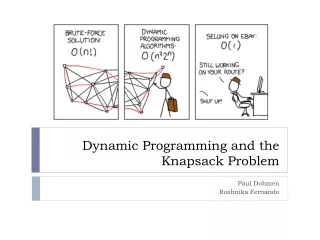
CS 332 - Algorithms Dynamic programming 0-1 Knapsack problem
CS 332 - Algorithms Dynamic programming 0-1 Knapsack problem. Review: Dynamic programming. DP is a method for solving certain kind of problems DP can be applied when the solution of a problem includes solutions to subproblems We need to find a recursive formula for the solution

CS 332 - Algorithms Dynamic programming 0-1 Knapsack problem
E N D
Presentation Transcript
CS 332 - Algorithms Dynamic programming 0-1 Knapsack problem
Review: Dynamic programming • DP is a method for solving certain kind of problems • DP can be applied when the solution of a problem includes solutions to subproblems • We need to find a recursive formula for the solution • We can recursively solve subproblems, starting from the trivial case, and save their solutions in memory • In the end we’ll get the solution of the whole problem
Properties of a problem that can be solved with dynamic programming • Simple Subproblems • We should be able to break the original problem to smaller subproblems that have the same structure • Optimal Substructure of the problems • The solution to the problem must be a composition of subproblem solutions • Subproblem Overlap • Optimal subproblems to unrelated problems can contain subproblems in common
Review: Longest Common Subsequence (LCS) • Problem: how to find the longest pattern of characters that is common to two text strings X and Y • Dynamic programming algorithm: solve subproblems until we get the final solution • Subproblem: first find the LCS of prefixes of X and Y. • this problem has optimal substructure: LCS of two prefixes is always a part of LCS of bigger strings
Review: Longest Common Subsequence (LCS) continued • Define Xi, Yj to be prefixes of X and Y of length i and j; m = |X|, n = |Y| • We store the length of LCS(Xi, Yj) in c[i,j] • Trivial cases: LCS(X0 , Yj ) and LCS(Xi, Y0) is empty (so c[0,j] = c[i,0] = 0 ) • Recursive formula for c[i,j]: c[m,n] is the final solution
Review: Longest Common Subsequence (LCS) • After we have filled the array c[ ], we can use this data to find the characters that constitute the Longest Common Subsequence • Algorithm runs in O(m*n), which is much better than the brute-force algorithm: O(n 2m)
0-1 Knapsack problem • Given a knapsack with maximum capacity W, and a set S consisting of n items • Each item i has some weight wi and benefit value bi(all wi , biand W are integer values) • Problem: How to pack the knapsack to achieve maximum total value of packed items?
W = 20 0-1 Knapsack problem:a picture Weight Benefit value bi wi Items 3 2 This is a knapsack Max weight: W = 20 4 3 5 4 8 5 10 9
0-1 Knapsack problem • Problem, in other words, is to find • The problem is called a “0-1” problem, because each item must be entirely accepted or rejected. • Just another version of this problem is the “Fractional Knapsack Problem”, where we can take fractions of items.
0-1 Knapsack problem: brute-force approach Let’s first solve this problem with a straightforward algorithm • Since there are n items, there are 2n possible combinations of items. • We go through all combinations and find the one with the most total value and with total weight less or equal to W • Running time will be O(2n)
0-1 Knapsack problem: brute-force approach • Can we do better? • Yes, with an algorithm based on dynamic programming • We need to carefully identify the subproblems Let’s try this: If items are labeled 1..n, then a subproblem would be to find an optimal solution for Sk = {items labeled 1, 2, .. k}
Defining a Subproblem If items are labeled 1..n, then a subproblem would be to find an optimal solution for Sk = {items labeled 1, 2, .. k} • This is a valid subproblem definition. • The question is: can we describe the final solution (Sn) in terms of subproblems (Sk)? • Unfortunately, we can’t do that. Explanation follows….
w1 =2 b1 =3 w2 =4 b2 =5 w3 =5 b3 =8 w4 =3 b4 =4 w1 =2 b1 =3 w2 =4 b2 =5 w3 =5 b3 =8 w4 =9 b4 =10 Defining a Subproblem Weight Benefit wi bi Item # ? 1 2 3 Max weight: W = 20 For S4: Total weight: 14; total benefit: 20 S4 2 3 4 S5 3 4 5 4 5 8 5 9 10 Solution for S4 is not part of the solution for S5!!! For S5: Total weight: 20 total benefit: 26
Defining a Subproblem (continued) • As we have seen, the solution for S4 is not part of the solution for S5 • So our definition of a subproblem is flawed and we need another one! • Let’s add another parameter: w, which will represent the exact weight for each subset of items • The subproblem then will be to compute B[k,w]
Recursive Formula for subproblems • Recursive formula for subproblems: • It means, that the best subset of Sk that has total weight w is one of the two: 1) the best subset of Sk-1 that has total weight w, or 2) the best subset of Sk-1 that has total weight w-wk plus the item k
Recursive Formula • The best subset of Sk that has the total weight w, either contains item k or not. • First case: wk>w. Item k can’t be part of the solution, since if it was, the total weight would be > w, which is unacceptable • Second case: wk <=w. Then the item kcan be in the solution, and we choose the case with greater value
0-1 Knapsack Algorithm for w = 0 to W B[0,w] = 0 for i = 0 to n B[i,0] = 0 for w = 0 to W if wi <= w // item i can be part of the solution if bi + B[i-1,w-wi] > B[i-1,w] B[i,w] = bi + B[i-1,w- wi] else B[i,w] = B[i-1,w] else B[i,w] = B[i-1,w] // wi > w
Running time O(W) for w = 0 to W B[0,w] = 0 for i = 0 to n B[i,0] = 0 for w = 0 to W < the rest of the code > Repeat n times O(W) What is the running time of this algorithm? O(n*W) Remember that the brute-force algorithm takes O(2n)
Example Let’s run our algorithm on the following data: n = 4 (# of elements) W = 5 (max weight) Elements (weight, benefit): (2,3), (3,4), (4,5), (5,6)
Example (2) i 0 1 2 3 4 W 0 0 1 0 2 0 3 0 4 0 5 0 for w = 0 to W B[0,w] = 0
Example (3) i 0 1 2 3 4 W 0 0 0 0 0 0 1 0 2 0 3 0 4 0 5 0 for i = 0 to n B[i,0] = 0
Items: 1: (2,3) 2: (3,4) 3: (4,5) 4: (5,6) Example (4) i 0 1 2 3 4 W 0 0 0 0 0 0 i=1 bi=3 wi=2 w=1 w-wi =-1 1 0 0 2 0 3 0 4 0 5 0 if wi <= w // item i can be part of the solution if bi + B[i-1,w-wi] > B[i-1,w] B[i,w] = bi + B[i-1,w- wi] else B[i,w] = B[i-1,w] else B[i,w] = B[i-1,w]// wi > w
Items: 1: (2,3) 2: (3,4) 3: (4,5) 4: (5,6) Example (5) i 0 1 2 3 4 W 0 0 0 0 0 0 i=1 bi=3 wi=2 w=2 w-wi =0 1 0 0 2 0 3 3 0 4 0 5 0 if wi <= w// item i can be part of the solution if bi + B[i-1,w-wi] > B[i-1,w] B[i,w] = bi + B[i-1,w- wi] else B[i,w] = B[i-1,w] else B[i,w] = B[i-1,w] // wi > w
Items: 1: (2,3) 2: (3,4) 3: (4,5) 4: (5,6) Example (6) i 0 1 2 3 4 W 0 0 0 0 0 0 i=1 bi=3 wi=2 w=3 w-wi=1 1 0 0 2 0 3 3 0 3 4 0 5 0 if wi <= w// item i can be part of the solution if bi + B[i-1,w-wi] > B[i-1,w] B[i,w] = bi + B[i-1,w- wi] else B[i,w] = B[i-1,w] else B[i,w] = B[i-1,w] // wi > w
Items: 1: (2,3) 2: (3,4) 3: (4,5) 4: (5,6) Example (7) i 0 1 2 3 4 W 0 0 0 0 0 0 i=1 bi=3 wi=2 w=4 w-wi=2 1 0 0 2 0 3 3 0 3 4 0 3 5 0 if wi <= w// item i can be part of the solution if bi + B[i-1,w-wi] > B[i-1,w] B[i,w] = bi + B[i-1,w- wi] else B[i,w] = B[i-1,w] else B[i,w] = B[i-1,w] // wi > w
Items: 1: (2,3) 2: (3,4) 3: (4,5) 4: (5,6) Example (8) i 0 1 2 3 4 W 0 0 0 0 0 0 i=1 bi=3 wi=2 w=5 w-wi=2 1 0 0 2 0 3 3 0 3 4 0 3 5 0 3 if wi <= w// item i can be part of the solution if bi + B[i-1,w-wi] > B[i-1,w] B[i,w] = bi + B[i-1,w- wi] else B[i,w] = B[i-1,w] else B[i,w] = B[i-1,w] // wi > w
Items: 1: (2,3) 2: (3,4) 3: (4,5) 4: (5,6) Example (9) i 0 1 2 3 4 W 0 0 0 0 0 0 i=2 bi=4 wi=3 w=1 w-wi=-2 1 0 0 0 2 0 3 3 0 3 4 0 3 5 0 3 if wi <= w // item i can be part of the solution if bi + B[i-1,w-wi] > B[i-1,w] B[i,w] = bi + B[i-1,w- wi] else B[i,w] = B[i-1,w] elseB[i,w] = B[i-1,w]// wi > w
Items: 1: (2,3) 2: (3,4) 3: (4,5) 4: (5,6) Example (10) i 0 1 2 3 4 W 0 0 0 0 0 0 i=2 bi=4 wi=3 w=2 w-wi=-1 1 0 0 0 2 0 3 3 3 0 3 4 0 3 5 0 3 if wi <= w // item i can be part of the solution if bi + B[i-1,w-wi] > B[i-1,w] B[i,w] = bi + B[i-1,w- wi] else B[i,w] = B[i-1,w] elseB[i,w] = B[i-1,w]// wi > w
Items: 1: (2,3) 2: (3,4) 3: (4,5) 4: (5,6) Example (11) i 0 1 2 3 4 W 0 0 0 0 0 0 i=2 bi=4 wi=3 w=3 w-wi=0 1 0 0 0 2 0 3 3 3 0 3 4 4 0 3 5 0 3 if wi <= w// item i can be part of the solution if bi + B[i-1,w-wi] > B[i-1,w] B[i,w] = bi + B[i-1,w- wi] else B[i,w] = B[i-1,w] else B[i,w] = B[i-1,w] // wi > w
Items: 1: (2,3) 2: (3,4) 3: (4,5) 4: (5,6) Example (12) i 0 1 2 3 4 W 0 0 0 0 0 0 i=2 bi=4 wi=3 w=4 w-wi=1 1 0 0 0 2 0 3 3 3 0 3 4 4 0 3 4 5 0 3 if wi <= w// item i can be part of the solution if bi + B[i-1,w-wi] > B[i-1,w] B[i,w] = bi + B[i-1,w- wi] else B[i,w] = B[i-1,w] else B[i,w] = B[i-1,w] // wi > w
Items: 1: (2,3) 2: (3,4) 3: (4,5) 4: (5,6) Example (13) i 0 1 2 3 4 W 0 0 0 0 0 0 i=2 bi=4 wi=3 w=5 w-wi=2 1 0 0 0 2 0 3 3 3 0 3 4 4 0 3 4 5 0 3 7 if wi <= w// item i can be part of the solution if bi + B[i-1,w-wi] > B[i-1,w] B[i,w] = bi + B[i-1,w- wi] else B[i,w] = B[i-1,w] else B[i,w] = B[i-1,w] // wi > w
Items: 1: (2,3) 2: (3,4) 3: (4,5) 4: (5,6) Example (14) i 0 1 2 3 4 W 0 0 0 0 0 0 i=3 bi=5 wi=4 w=1..3 1 0 0 0 0 0 2 0 3 3 3 3 0 3 4 4 4 0 3 4 5 0 3 7 if wi <= w // item i can be part of the solution if bi + B[i-1,w-wi] > B[i-1,w] B[i,w] = bi + B[i-1,w- wi] else B[i,w] = B[i-1,w] elseB[i,w] = B[i-1,w]// wi > w
Items: 1: (2,3) 2: (3,4) 3: (4,5) 4: (5,6) Example (15) i 0 1 2 3 4 W 0 0 0 0 0 0 i=3 bi=5 wi=4 w=4 w- wi=0 1 0 0 0 0 0 2 0 3 3 3 3 0 3 4 4 4 0 3 4 5 5 0 3 7 if wi <= w// item i can be part of the solution if bi + B[i-1,w-wi] > B[i-1,w] B[i,w] = bi + B[i-1,w- wi] else B[i,w] = B[i-1,w] else B[i,w] = B[i-1,w] // wi > w
Items: 1: (2,3) 2: (3,4) 3: (4,5) 4: (5,6) Example (15) i 0 1 2 3 4 W 0 0 0 0 0 0 i=3 bi=5 wi=4 w=5 w- wi=1 1 0 0 0 0 0 2 0 3 3 3 3 0 3 4 4 4 0 3 4 5 5 0 3 7 7 if wi <= w// item i can be part of the solution if bi + B[i-1,w-wi] > B[i-1,w] B[i,w] = bi + B[i-1,w- wi] else B[i,w] = B[i-1,w] else B[i,w] = B[i-1,w] // wi > w
Items: 1: (2,3) 2: (3,4) 3: (4,5) 4: (5,6) Example (16) i 0 1 2 3 4 W 0 0 0 0 0 0 i=3 bi=5 wi=4 w=1..4 1 0 0 0 0 0 0 2 0 3 3 3 3 3 0 3 4 4 4 4 0 3 4 5 5 5 0 3 7 7 if wi <= w // item i can be part of the solution if bi + B[i-1,w-wi] > B[i-1,w] B[i,w] = bi + B[i-1,w- wi] else B[i,w] = B[i-1,w] else B[i,w] = B[i-1,w]// wi > w
Items: 1: (2,3) 2: (3,4) 3: (4,5) 4: (5,6) Example (17) i 0 1 2 3 4 W 0 0 0 0 0 0 i=3 bi=5 wi=4 w=5 1 0 0 0 0 0 0 2 0 3 3 3 3 3 0 3 4 4 4 4 0 3 4 5 5 5 0 3 7 7 7 if wi <= w// item i can be part of the solution if bi + B[i-1,w-wi] > B[i-1,w] B[i,w] = bi + B[i-1,w- wi] else B[i,w] = B[i-1,w] else B[i,w] = B[i-1,w] // wi > w
Comments • This algorithm only finds the max possible value that can be carried in the knapsack • To know the items that make this maximum value, an addition to this algorithm is necessary • Please see LCS algorithm from the previous lecture for the example how to extract this data from the table we built
Conclusion • Dynamic programming is a useful technique of solving certain kind of problems • When the solution can be recursively described in terms of partial solutions, we can store these partial solutions and re-use them as necessary • Running time (Dynamic Programming algorithm vs. naïve algorithm): • LCS: O(m*n) vs. O(n * 2m) • 0-1 Knapsack problem: O(W*n) vs. O(2n)