
Download

1 / 0
Download Presentation 
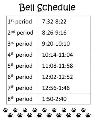
Bell Schedule
An Image/Link below is provided (as is) to download presentation
Download Policy: Content on the Website is provided to you AS IS for your information and personal use and may not be sold / licensed / shared on other websites without getting consent from its author.
Content is provided to you AS IS for your information and personal use only.
Download presentation by click this link.
While downloading, if for some reason you are not able to download a presentation, the publisher may have deleted the file from their server.
During download, if you can't get a presentation, the file might be deleted by the publisher.
E N D
Presentation Transcript
- Developing the school bell schedule can be a very complex task especially when incorporating shortened days for staff development, assembly schedules, rotating schedules, block schedules, mandated testing schedules and final exam schedules while at the same time keeping track of the total instructional minutes to meet state and contractual requirements. This tool is an Excel spreadsheet that automates the counting of the number of instructional minutes and days in the school year. This allows you to be as creative as you want and experiment with multiple bell schedules until you find the perfect one. All of the formulas used in this spreadsheet are visible so you are able to learn how the spreadsheet works, but be careful; if you delete a formula, the spreadsheet will not work correctly. A basic understanding of Excel and working with formulas in Excel is recommended to use this tool, but don’t worry, these instructions will provide you with the basics of working with Excel and formula writing to get you started. So… let’s get started!!
Bell Schedule
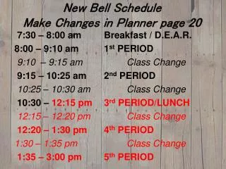
Click to proceed - When you first open the Bell Schedule spreadsheet, you will see the “Count Balance” calculation area at the top left of the page If you click on cell E1 (the one with the number 180) you will see this in the Formula Bar Here is the formula - this is the typical structure of an Excel formula =SUM(C18+C61+L61+R61+L19+R19+X61+X19+C103+L105+C143+L143) Back Click to proceed
- We will get back to that formula in a minute. Let’s take a look at the structure of formulas with a couple of examples: Click on an empty cell somewhere on the spreadsheet – G10 would be a good one to use Enter an equal sign “=“ (no quotes) in the cell – typically, formulas in Excel begin with an equal sign After the equal sign, type in the number 180, then type the multiply sign (the asterisk) and then type the number 360. Your formula should look like this: =180*360 Then press Enter – did you get 64800? GREAT!! This number (64800) is the number of instructional minutes per year currently (2013) required by the state of California in public high schools. As you can see, this number is used in cell E3 as a constant to evaluate the instructional minutes of the bell schedule you create. Let’s take a look at one more example… Back Click to proceed
- Click on cell G10 and enter the number 180 (this will erase the formula you entered in the previous example, but that is what we want to do Click on cell G11 and enter the number 360 Click on cell G12 and enter the following formula: =G10*G11 Press the Enter key – Did you get 64800 again? GREAT!! This method of entering formulas by referencing cells that contain constants instead of imbedding constants within formulas is a far superior way of writing formulas – a lesson that was clearly demonstrated at the turn of the millennium. You will see that this preferred method is used throughout the Bell Schedule spreadsheet. (Go back and delete your entries in cells G10, G11 and G12) Getting back to the formula in cell E1: =SUM(C18+C61+L61+R61+L19+R19+X61+X19+C103+L105+C143+L143) The formula says to calculate the sum of the contents of the cells at C18, C61, L61, R61, L19, R19, X61, X19, C103, L105, C143 and L143. Go to each of these cells on the spreadsheet to see what’s there and check to see if the sum is correct. Did it add up to 180? GREAT!! Did you write the numbers on a piece of paper and add them up or did you use your new formula writing skills in some blank cells on the Excel spreadsheet?? Either way is fine!! Now let’s get to bell scheduling!! Back Click to proceed
- Getting Oriented 4 1 3 2 This is a reduced view of the entire spreadsheet. You have already seen the “Count Balance” area on the top left. The rest of the spreadsheet is composed of 12 individual bell schedule calculation areas. These bell schedules are identical in format, but differ in the use of time. For example, schedule 1 is a traditional schedule, the combination of schedules 2 and 3 make up an AB rotating block schedule, add schedule 4 to this and you can develop an AB block schedule that banks time for a weekly, one-hour staff development period. Let’s take a closer look at bell schedule 1. 5 6 7 8 9 10 11 12 Back Click to proceed
- A Closer Look The Data Entry Section: Your bell schedule parameters are entered here The Bell Schedule Section: The bell schedule resulting from the data entered above appears here Back Click to proceed
- The Details of the Data Entry Section Minute Calculation Formulas These calculations are used to compute time in the bell schedule. The 1440 is the number of minutes in one day. The decimal fraction is the number of minutes entered for the length of a component divided by 1440. This fraction is used in the Bell Schedule Section. I’m sure there is a better way to do this, but it is what I came up with a long time ago and it works. The starting time of school, the number of minutes for each bell schedule component and the number of days on this schedule is entered in this column. The titles can all be changed to meet individual needs and zeros or blanks can be used for components not used. If needed, additional categories can be added but make sure that the cell containing the number of the “Days on this schedule” is contained in the formula in cell E1. Also be sure to copy and paste the “Minute Calculation Formulas” in the appropriate places of the newly added categories (I’ll show you how to do this later on in this guide). Back Click to proceed
- Structure of the Bell Schedule Section The formulas in this column add 2 numbers: 1) the number of minutes specified in the Data Entry Section for the particular schedule component and 2) the starting time of the component. This sum gives the ending time. This is a formula that copies the starting time of school you entered in the Data Entry Section above. This formula (and all the others below it in this column) just copy the ending time of the previous bell schedule component. This column calculates the number of minutes for each component as a double check and for adding the total instructional minutes. Back Click to proceed
- Structure of the Bell Schedule Section - continued The Total Instructional Minutes A B C D E This is the formula that calculates the total instructional minutes in cell E43: =SUM(E26:E38)-(E34)-(E29) This formula calculates the sum of the numbers in the “E” column from row 26 through 38 and then subtracts the numbers in cell “E34” (Lunch) and “E29” (Break) – minutes that don’t usually count as instructional. Notice that only 6 class periods are included. What do you do if you are on a 7 period day? Adjust the formula in cell E43. Change the formula to read: =SUM(E26:E40)-(E34)-(E29) (Red added for emphasis only) Back Click to proceed
- Structure of the Bell Schedule Section - continued Any of the categories in this column can be changed as needed. Additional categories can be added here. The next slide will guide you through this process. Back Click to proceed
- Adding Components to a Bell Schedule IMPORTANT!! Save a copy of the spreadsheet before you make any changes – just in case. You will be making two types of additions to a bell schedule: 1) adding components to blank spaces that already exist in the spreadsheet and 2) creating blank spaces where there were none. Let’s start with the first case. Let’s say that you are on a 9 period day. You can change the titles in the first column to look like this – Just type in whatever you need in the cells of this column. Next we will deal with the formulas. Back Click to proceed
- Adding Components to a Bell Schedule - continued There are only 3 different formulas used to produce the bell schedule: one that copies the starting time of school, one that copies the ending time of one period to the next period’s start time and one that adds the bell schedule component minutes to the starting time. Let’s take a look at these: The formula in cell C24 is: =C10 All this does is make cell C24 equal to whatever time is entered in cell C10 – here the time 6:46 AM The rest of the formulas in this column all to the same thing – copy the ending time of the previous period – here is the formula in cell C27: =D26. Taking a look at these two cells you will see the same time – 8:47 AM Back Click to proceed
- Adding Components to a Bell Schedule - continued Now let’s take a look at the formulas that really make this all work – in this example the cells in column D, the “END” column, cells 24 through 40. These are the cells that add the bell schedule component minutes from the Data Entry Section to the starting time of the period. The formula in cell D24 is: =C24+E12 This takes the time entered in cell C24 (6:46 AM) and adds the minutes assigned to the length of first period (57 minutes). Remember – the formula uses the calculation result in column “E”, not the time entered in column “C”. You don’t have this exact bell schedule example in the Excel spreadsheet, but if you look at the formulas in any of the “END” columns, you can see how this all works. By changing the column “E” reference in the formula, you assign the times listed in the Data Entry Section. Back Click to proceed
- Adding Components to a Bell Schedule - continued Did you notice when I showed you the example of changing to a 9 period day that I didn’t really finish the job? Well, let’s take care of that now. This involves adding formulas, which isn’t that big of a deal if you just follow the pattern or copy formulas DOWN. Let’s look at cell C41: Remember, this column copies the “END” time from the previous period. You could just follow the pattern and enter the following: =D40 This would copy the time of 3:54 PM to cell C41. Another method would be to select cell C40, click on “Copy”, click on cell C41, click on “Paste” and then press “Enter”. Both methods work just fine. I prefer the copy and paste method (with a slight variation) and I’ll show you why on the nextslide. Back Click to proceed
- Adding Components to a Bell Schedule - continued Instead of copying and pasting just one cell at a time, I prefer to do it all at once. Start by selecting all three cells that you need to copy – in this example C40, D40 and E40. This is done by clicking on cell C40, holding the click down and dragging over cells D40 and E40, then releasing the click. It should look like this: Take note of this little darkened square – next we will use this to paste down the formulas. Back Click to proceed
- Adding Components to a Bell Schedule - continued In Excel, the cursor normally looks something like this: When you move the cursor on top of the little solid square, it changes to look something like this: While the cursor appears in this solid plus-sign mode, click and drag down to cell E42 (for this example) and then release the click. This will copy DOWN the “C” column formulas in the “C” column, the “D” column formulas in the “D” column and the “E” column formulas in the “E” column. The formulas in the “C” and “E” columns will be exactly what you want, but the formulas in the “D” column will have to be adjusted. We will see why in the next slide. Back Click to proceed
- When copying cells and pasting them in a new location (like we just did) Excel tries to follow a pattern. Since the formulas in the columns “C” and “E” follow a pattern, these cells are pasted in exactly like we want them. Since the formulas in the “D” column reference various times in the Data Entry Section, these formulas need to be adjusted. This is accomplished by looking at the Data Entry Section and finding the row with the correct time element for the specific period and then changing the reference in the “D” column. Let’s see how this looks: REMINDER: Use THIS column of numbers for the formulas to calculate the END time of a period. The formula at D41: =C41 + E12 is obviously incorrect. It references an instructional period length, not the length of a passing period. To fix this, click on cell D41 and change the E12 in the formula to E14 and press enter. The new formula looks like this: =C41 + E14 and the 57 minutes changes to 7 B C D E Back Click to proceed
- Here is a look at the final schedule, but there is still one more formula to adjust, the TOTAL INSTRUCTIONAL MINUTES – Cell E43 This formula was set to count the instructional minutes before we added periods to the day – so we need to adjust the formula to count the new periods. The current formula is: =SUM(E26:E38)-(E34)-(E29) This formula starts counting instructional minutes at period 2 and ends at period 7 – a 6-period day. If you want it to include all 9 periods, change E26 to E24 and change E38 to E42. The new formula will look like this: =SUM(E24:E42)-(E34)-(E29) This formula says: sum all the numbers from cell E24 through E42 and subtract the numbers in cell E34 and E29 Back Click to proceed
- Using a combination of the 12 Bell Schedule Calculation areas in the spreadsheet and what you have learned so far, you should be able to manipulate the schedules to come up with the bell schedule you need. But there may be a need to add another row to a bell schedule when there are no blank spaces to do this. No problem!! Select the entire row where you need cells added including the one cell to the left of the “PERIOD” column (in this example cell A42). This needs to be done to keep entries further down in this column aligned properly Click on Insert in the Task Bar and select Insert Cells 3) This dialog box will appear asking how you want the cells inserted – the “Shift cells down” choice is what you want for this example. Click on OK Back Click to proceed
- Now you have a blank row in the bell schedule to add whatever you need When you add cells like this, Excel does a couple of very nice things automatically for you. Notice that the “TOTAL INSTRUCTIONAL MINUTES” formula moves from cell E43 to cell E44, but does the calculation include the newly created row? YES!! The formula changes it’s calculation range to include the new row. (It also adjusts any other calculations on the spreadsheet that moved as a result of the addition of cells) Another automatic change is in the “Count Balance” calculation area at the top left of the spreadsheet. These formulas are automatically changed to account for the movement of cells. 44 Back Click to proceed
- This is the “Count Balance” calculation area at the top left of the spreadsheet E1 E4 A Word of Caution: If you insert cells/move the location of cells on the spreadsheet, make sure that the formulas at E1 and E4 of the “Count Balance” calculation area contain the correct references to the cells on the individual Bell Schedule that contain the number of “Days on this schedule” and “Total Instructional Minutes” (in this example – cell C18 for the “Days on this schedule” and cell E44 for the “Total Instructional Minutes”). When you add cells using the above procedure, Excel takes care of the formula adjustments, but I always check! C18 E44 The “Count Balance” calculation area is copied below each of the 12 Bell Schedules for convenience – you don’t have to go back to the top of the spreadsheet to see the overall effect of a change. 180 Back 64,800 0 Click to proceed
- Now you’re ready to start developing a complete bell schedule. We will begin with a short example to create a rotating, A B block schedule. When you first open the Bell Schedule spreadsheet, it is set up with a fairly traditional bell schedule that banks minutes for 4 days per week and uses the banked minutes on one day per week for staff development. It also contains testing days and two different assembly days. The complete bell schedule is made by combining information from bell schedules 1, 5, 9, 10, 11 and 12. Take a look at these schedules to see how they combine to make the complete bell schedule. Ok – now you want to get rid of this schedule to make our example rotating, block A B schedule. Be sure to work on a copy, just in case. It’s very easy to get rid of this schedule – all you have to do is delete the “Days on this schedule” number on each of the schedules listed above. These numbers are at cells C18, C61, C103, L105, C143 and L143. Go to each of these cells and delete the numbers in the cell (leave the cells blank). Back Click to proceed
- The “Count Balance” calculation area should now look like this: Now go over to Bell Schedules 2 and 3 located in the area from J7 to T32. We will use these two schedules to make our AB block schedule. Back Click to proceed
- Start with the Block Schedule A We arbitrarily set the starting time of school to be 7:50 AM (any time can be used). In the blank spaces of the “L” column enter the following: L11 – 86 L12 – 86 L13 – 86 L14 – 86 L15 – 5 L16 – 40 L17 – 10 L18 – 6 L19 - 90 The “L” column will now look like this Back Click to proceed
- Now move to the Block Schedule B In the blank spaces of the “R” column enter the same numbers you entered in the Block Schedule A: R11 – 86 R12 – 86 R13 – 86 R14 – 86 R15 – 5 R16 – 40 R17 – 10 R18 – 6 R19 - 90 The “R” column will now look like this Back Click to proceed
- Now take a look at the “Count Balance” calculation area. You have a schedule with 180 days and exactly the required instructional minutes. ALWAYS do a little checking to make sure!! Are the “Days on this schedule” numbers at L19 and R19 included in the formula at E1? (With E1 equal to 180 it is a good bet that everything is OK. Are the “Total Instructional Minutes” formulas at cells N43 and T43 calculating the correct minutes from the schedule? Do you find (L19*N43) and (R19*T43) in the formula at cell E4? Always perform these checks to make sure your schedule is making the correct calculations. Back Click to proceed
- Now for the final example, let’s get a bit more creative. You want to create an AB rotating, block schedule, but you want to bank minutes so you can have one hour of staff development time one day each week. To do this, add in Bell Schedule 4. Try this on your own to see if you can come up with a workable schedule. I will start you off with a hint: Change the number of days on the A and B schedule to 75 each and set the number of days on Bell Schedule 4 to 30. Now just enter times in column “X” and keep adjusting times in columns “L”, “R” and “X” until you get a working solution. Change to 75 Set at 30 A working solution (one of many) is on the next 2 pages – so you can either go ahead and see one solution or play on your own to come up with one. Back Click to proceed
- These are the A and B schedules that bank time and would be in place 4 days per week. The schedule utilizing the banked minutes for staff development is on the next page. Back Click to proceed
- This is the schedule in place one day per week that utilizes the banked minutes for staff development Be sure to do the formula checking!! Back Click to proceed
- You now have a working understanding of how to use the Bell Schedule spreadsheet. Remember to always keep the original spreadsheet unchanged and work only with copies. Finally, always check the formulas!! You don’t want to start the school year and then find out that your instructional minutes are incorrect. If you have suggestions for improvements, please contact us using the information below. Thank you and happy scheduling!! The Bell Schedule spreadsheet and these instructions are provided to you at no cost by the College & Career Academy Support Network (CCASN) Since 1998 CCASN has been working to increase educational opportunities that offer each young person support and guidance, productive engagement in the world outside of school, and preparation for both college and careers. This research-based strategy has been effective for hundreds of thousands of teenagers, including low-income students of color. CCASN offers professional development, coaching, resource materials, and technical assistance for secondary educators, schools, and districts. Visit the CCASN web site at: http://casn.berkeley.edu College & Career Academy Support Network (CCASN)University of California. Berkeley · Irvine1608 Tolman HallBerkeley, CA 94720-1670 Phone: 510-643-5748FAX: 510-642-2124 Back Click to Exit


More Related