Download
1 / 35
390 likes | 583 Views
Ch.7 The z-Transform and Discrete-Time Systems. 7.1 The z-Transform. Definition: Consider the DTFT: X( Ω ) = Σ all n x[n]e -j Ω n (7.1) Now consider a real number ρ and the factor ρ n Then X(z) = Σ all n x[n] ρ -n e -j Ω n = Σ all n x[n]z -n

E N D
7.1 The z-Transform • Definition: • Consider the DTFT: X(Ω) = Σall nx[n]e -jΩn (7.1) • Now consider a real number ρ and the factor ρn • Then X(z) = Σall nx[n] ρ-n e -jΩn= Σall nx[n]z-n • Where z is the complex number ρe-jΩ . • This is the two-sided z-transform. • The one-sided z-transform has n=0,…,∾ • In this text, the one-sided z-transform is assumed.
Example 7.1 z-transform of the Unit Pulse • Let x[n] = δ(n) = {1 for n=0 and 0 otherwise}. • Then X(z) = Σn≥0x[n]z-n =δ(0) z0 = 1 (7.6) • So: δ(0) ↔ 1 • And the region of convergence is all z, where z is a complex number.
Example 7.2 z-transform of a Shifted Unit Pulse • Let x[n] = δ(n-q) • Then X(z) = Σn≥0x[n]z-n =δ(0) z-q = z-q • So: δ(n-q) ↔ z-q =1/ zq • And the region of convergence is all z except for z=0.
Example 7.3 Unit-Step Function • Consider x[n] = u[n] = {1 n≥0; 0 otherwise} • X(z) = U(z) = Σn≥0x[n]z-n = Σn≥0z-n • So: U(z) = 1 + z-1 + z-2 … • Now (z-1)U(z) = (z+1+z-1 + z-2 …) – (1+z-1 + z-2 …) • And U(z) = z/(z-1) • So: U(z) ↔ z/(z-1 )= 1/(1-z-1) • And the region of convergence will be |z|>1.
Example 7.4 z-transform of anu[n] • Let x[n] = anu[n] • Then X(z) = Σn≥0 anz-n =(1 + az-1 +a2 z-2 …) • Now (z-a)X(z) =(z + a +a2 z-1 …) - (a + a2z-1 +a3 z-2 …) • And X(z) = z/(z-a) • So X(z) ↔ z/(z-a) = 1/(1-az-1) • With the region of convergence |z|> |a| and a is any real or complex number.
7.1.1 Relationship between the DTFT and the z-transform • X(Ω) = X(z) with z = ejΩ only when the region of convergence includes the unit circle, ie |z|=1.
Properties of the z-Transform • Linearity—Example 7.5 • Let x[n] = u[n] and v[n] = anu[n], where a≠1 • Now u(n) ⟷ z/(z-1) and anu[n]⟷ z/(z-a) • So x[n] + v[n] ⟷ z/(z-1) + z/(z-a) = • (2z2 – (1 + a)z/(z-1)(z-a)
Example 7.6 z-Transform of a Pulse • Using the right shift property: • x[n-q]u[n-q]⟷ z-q X(z) • Let p[n] = u[n] – u[n-q] be a pulse of 1’s from n=0 to n= (q-1) and u[n-q]=1n-qu[n-q] • Now u(n)⟷z/(z-1) and u[n-q]⟷z-q(z/z-1) • So p[n]⟷z/(z-1)-z-q(z/z-1)=(zq-1)/zq-1(z-1)
Example 7.8 z-Transform of nanu[n] • Let x[n] = nanu[n]; then anu[n] ⟷ z/(z-a) • Also, the property of “multiplication by n” • nx[n] ⟷ -z (d/dz X(z)) • So taking the derivative • d/dz (z/z-a)=1/(z-a) –z/(z-a)2=-a/(z-a)2 • And using the properties: • n anu[n] ⟷ -z (-a)/(z-a)2 = az/(z-a)2 • And for a=1 we have nu[n]⟷ z /(z-1)2
Example 7.11 z-Transform of Sinusoids • Let v[n] = (cos Ωn) u[n] • The property of multiplication by sinusoid • (cos Ωn)x(n) ⟷ (1/2) { X(ejΩz) + X(e–jΩz)} • Using the property • After “manipulation” we have • (cos Ωn) u[n]⟷ z2 – (cosΩ)z/(z2-(2cosΩ)z + 1) • Similarly it can be shown: • (sin Ωn) u[n]⟷ (sinΩ)z/(z2-(2cosΩ)z + 1)
Other Properties • Summation • Convolution • Initial-Value Theorem • Final-Value Theorem
7.3 Computation of the Inverse z-Transform • Complex integral, with integration taken along a counterclockwise close circular contour that is contained in the region of convergence. • When X(z) is a rational function then we can be computed by expansion of X(z) into a power series in z-1.
Example 7.15 Inverse z-Transform via Long Division • Let X(z) = (z2 -1)/(z3 + 2z +4) • Then by long division we have: • X(z) = z-1 -3z-3 – 4 z-4 … • And by the definition of the z-transform • x[0] = 0; x[1] = 1; x[2]= 0; x[3] =-3; x[4] =-4; …
Inversion via Partial Fraction Expansion • Suppose X(z) = B(z)/A(z) is a rational function. • If the degree of B(z) is equal to A(z) then dividing A(z) into B(z) yields X(z) = x[0] + R(z)/A(z). • But also, X(z)/z = B(z)/zA(z), which can be expanded into partial fractions.
Distinct Poles • Suppose the poles of X(z) are distinct: • X(z)/z = c0/z + c1/(z-p1) + …+cN/(z-pN) • Here c0 = {z X(z)/z} evaluated at z=0. • Also ci = {(z-pi)X(z)/z) evaluated at z=pi • Then X(z) = c0 + c1z/ (z-p1) + …+zcN/(z-pN) • And taking the inverse z-transform using the Table of Pairs • x[n] = c0δ(0)+ c1p1n + …+cNpNn
Complex Poles • If all the poles of X(z) are real, the terms comprising the signal are all real-valued. • If two or more poles are complex, the corresponding terms will be complex-valued. • These complex terms can be combined to yield real-valued terms; in this case the poles are complex conjugates. • If p1=a +jb is a complex pole, and p2 = a –jb is its complex conjugate then when added we have c1p1n + c1*p1*n which can be expressed as a real term: 2|c1|σn cos(Ωn + ∟c1). • Here c2 =c1*, σ = |p1|, and Ω=∟p1.
Example 7.17 Complex Poles • Let X(z) = (z3 +1)/(z3 – 2 –z -2) • Use the MATLAB command roots to find the poles p1 = -.05 – j0.866, p2 = -.5 + j0.866, and p3=2; or you could recognize that (z-2) is a factor of the denominator and then factor the denominator accordingly. • Since the order of the numerator and denominator are equal, X(z)/z is expanded. • c0, c1, c2, and c3 are found using the procedure outlined for “distinct poles”; also note c2=c1*. • The final result is: • x[n] = -0.5δ(n) + 0.874 cos(4/3 n + 10.89º) + 0.643(2)n
Repeated Poles • Discussed on pages 374-375. • The residues (ci’s) are computed in a similar fashion as shown in the distinct pole case. • Example 7.18 (p.375-376) illustrates the concepts.
Pole Location and the Form of the Signal • Relationships between signal poles and terms is similar to that in the Laplace Transform Theory. • In particular, x[n] converges to 0 as n→∾ if and only if all of the poles have magnitudes that are strictly less than 1 (lies inside the unit circle.)
7.4 Transfer Function Representation • First – Order Case • Let y[n] + ay[n-1] = bx[n] • Then take the z-transform to get: • Y(z) + a{ z-1Y(z) + y[-1] }= b X(z) • Simplifying: • Y(z) (1 + az-1) = b X(z)-a y[-1] • Y(z) = (b X(z)-a y[-1])/ (1 + az-1) • Y(z) ={ b X(z)/(1 + az-1)} – {a y[-1]}/ (1 + az-1) • If y[-1] =0 then: • Y(z) = b X(z)/(1 + az-1)= z b X(z)/(z + a) • And we have the transfer function H(z): • Y(z) = H(z) X(z) so H(z) = b z /(z + a)
Example 7.19 Step Response of a First Order System • Let x≠1 and x[n] = u[n]; Then X(z) = z/(z-1) • Let Y(z)={bX(z)/(1+az-1)} – {ay[-1]}/(1+az-1) from general result of a first-order system. • Then : • Y(z) ={ (z/z-1)b/(1 + az-1)} – {a y[-1]}/ (1 + az-1) • Y(z) ={ (z/z-1)bz/(z + a)} – {a y[-1]z}/ (z + a) • Y(z) ={ (bz2/(z-1)(z + a)} – {a y[-1]z}/ (z + a) • Now, expand the first term: • {bz2/(z-1)(z + a)}(1/z) = {ab/(a+1)(z+a)}+{b/(a+1)(z-1)}
Example 7.19 (cont.) • So we have: • Y(z) ={ (bz2/(z-1)(z + a)} – {a y[-1]z}/ (z + a) • Y(z) ={abz/(a+1)(z+a)}+{bz/(a+1)(z-1)}–{ay[-1]z}/(z+a) • Now we have the following pairs: • u[n] ↔ z/(z-1) • anu[n] ↔ z/(z-a)= z/(z+(-a)) • So taking the inverse z-transform of Y(z): • y[n] = {ab/(a+1)(-a)nu[n] }+b/(a+1)u[n] – ay[-1](-a)nu[n] • y[n] = {b/(a+1)}{-(-a)n+1 +1} – ay[-1](-a)n n=0,1,2,… • And if y[-1] =0 then • {b/(a+1)}{-(-a)n+1 +1} n=0,1,2…. (text is different)
7.4.2 Second-Order Case • Consider the following difference equation: • Y[n] +a1y[n-1] +a2y[n-2] = b0x[n] + b1x[n-1] • Result for y[n-1]=y[n-2] =0: • H(z) = (b0z2 + b1z)/(z2 + a1z + a2)
Example 7.20 Second-Order System • The general result for the second order system is given by equation 7.87. • For the case with the a1 = 1.5, a2 = .5, b0=1 and b1=-1 we have • y[n] = 0.5(-.05)n - 3(-1)n n=0,1,2,3,… • Note that the first term dies off but the second term continues (see fig. 7.2).
Nth Order Case • y[n] +a1y[n-1] +…+aNy[n-N] =b0x[n]+…+bMx[n-M] • And H(z) = B(z)/A(z) • Where H(z) =(b0+…+bMz-M)/(1 + a1z-1+ …+aNz-N) • Now multiply by (zN/zN) • H(z) = (b0zN +…+bMzN-M)/ (zN + a1zN-1 + …+ aN) • So we have • B(z) = (b0zN +…+bMzN-M) • A(z) = (zN + a1zN-1 + …+ aN)
7.4.4 Transform of the Input/Output Convolution Sum • Y(z) = H(z) X(z) where h[n] ↔ H(z). • Let H(z) = B(z)/A(z) • Then Y(z) = {B(z)/A(z)} X(z) • A causal liner time-invariant discrete-time system is said to be finite dimensional if the transfer function H(z) is a rational function of z.
Example 7.21 Computation of aTransfer Function Let h[n] = 3(2-n)cos(n/6 + /12) n=0,1,2,… Note that cos(a+b) = cos(a)cos(b) – sin(a)sin(b). So h[n] = 3(2-n){cos(n/6) cos(/12) - sin(n/6)sin(/12)} n=0,1,2,… And h[n] = 2.898(2-n)cos(/12) – 0.776(2-n)sin(n/6), n=0,1,2,… Taking the z-transform of h[n] gives: H(z) = (2.898 z2 – 1.449z)/(z2 - .866z + .25)
7.22 Computation of Step Response If x[n] = u[n] then X(z) = z/(z-1). Since Y(z) = H(z) X(z) the step response can be calculated as Y(z) = H(z) {z/(z-1)}. Page 384-386 gives the example of the step response for the system from example 7.21. Figure 7.3 illustrates the plot of the step response.
Transfer Function of Interconnections • Unit Delay • y[n] = x[n-1] • Y(z) = z-1 X(z)
Example 7.23 Computation of the Transfer Function of Interconnections • Consider a discrete time system given by Figure 7.23. • From the figure: • zQ1(z) = Q2(z) + X(z) • zQ2(z) = Q1(z) – 3Y(z) • Y(z) = 2Q1(z) + Q2(z)
Example 7.23 (cont.) • Solving for Y(z) from these equations gives: • Y(z) = {(2z-1 +1)/(z – z-1) } {z-1X(z) – 3Y(z)} + 2z-1X(z) • Then it can be shown that: • H(z) = (2z+1)/(z2 +3z +5)
7.5 System Analysis Using the Transfer Function Representation • Consider the general linear time-invariant discrete-time system with transfer function H(z). • Let H(Z) = B(z)/A(z) where B(z) is an Mth-order polynomial and A(z) is an Nth-order polynomial and M≤ N and the polynomials do not have any common factors.
7.5 (cont.) • The time variation of h[n] is directly determined by the poles of the system. • The system is considered stableif its unit-pulse response, h[n], converges to zero as n tends to infinity. • To be stable, the poles must lie inside the “open” unit disk, in the z-plane. • The system is marginally stable if the unit-pulse is bounded (non-repeated poles could lie on the unit circle. • The system is unstableif the magnitude of the unit pulse function grows without bound (one or more poles located outside the unit circle or one or more repeated poles on the unit circle).
7.5.1 Response to a Sinusoidal Input • Let x[n] = C cos (Ω0n), n = 0, ±1, ±2, … • Then y[n] = C|H(Ω0)| cos(Ω0n + ∟H(Ω0) ), n = 0, ±1, ±2, … • Note: this is the sinusoidal steady state; see page 392 for the “transient response”.