Download
1 / 34
350 likes | 497 Views
This presentation provides an insightful overview of Petri Nets, essential mathematical modeling tools for capturing the dynamics of discrete event systems. It covers the fundamental building blocks, including graphical representation, state-transition mechanisms, and event scheduling. Applications in software design, workflow management, and reliability engineering are highlighted. Additionally, the discussion includes analysis techniques such as reachability, liveness, and boundedness, alongside extensions like colored and timed Petri Nets, offering a robust framework for modeling complex systems.

E N D
Petri NetsAn Overview IE 680 Presentation April 30, 2007 Renata Kopach- Konrad
Overview • The building blocks of Petri Nets • An example • Analysis tools • Extensions • Elements of steady-state simulation theory for SPNs
What are Petri Nets? • Mathematical modeling tools that capture operational dynamics of discrete event systems • Graphical Representation • Modeling Language • State-transition mechanism • Event Scheduling mechanism Not this kind of Petri!
Applications • Software design • Workflow management • Data Analysis • Reliability Engineering
Suitable for Modeling • Concurrency • Synchronization • Precedence • Priority • Bottom up and top-down modeling
Modeling Tool: Petri Nets • Supports modularity and abstraction • Supports system simulation • Supports formal analysis for operational properties such as boundedness, liveness, reachabiltiy, etc. • Petri Nets have a rich research literature
p1 1 1 t1 p2 t2 p3 t3 2 1 1 1 1 p4 t4 2 1 What is a Petri Net?
p1 1 1 t1 p2 t2 p3 t3 2 1 1 1 1 p4 t4 2 1 System State: Tokens and Net Marking Mo=(M(p1), M(p2), M(p3), M(p4))=(1,1,2,1)
p1 1 1 t1 p2 t2 p3 t3 2 1 1 1 1 p4 t4 2 1 Initial State: (1,1,2,1) t2 is enabled
p1 1 1 t1 p2 t2 p3 t3 2 1 1 1 1 p4 t4 2 1 Fire t2, New State: (1,0,3,2)
p1 1 1 t1 p2 t2 p3 t3 2 1 1 1 1 p4 t4 2 1 Fire t3, New State: (2,0,2,2)
p1 p1 1 1 1 1 t1 t1 p2 p2 t2 t2 p3 p3 t3 t3 2 2 1 1 1 1 1 1 1 1 p4 p4 t4 t4 2 2 1 1 Fire t1, New State: (1,2,2,2)
Fire t4, New State: (1,3,2,0) p1 1 1 t1 p2 t2 p3 t3 2 1 1 1 1 p4 t4 2 1
In the context of DES • Marking of the SPN = state of the system • Firing of a transition = occurrence of an event
Notation… A Petri net is a 5-tuple , where • S is a set of places • T is a set of transitions • F is a set of arcs s.t. • M0is an initial marking • W is the set of arc weights/transition matrix/incidence matrix
…allows for many things The state of a net is an M vector so State equations are possible • Where is how many times each transition fires • WTstate transition matrix
p1 1 1 t1 p2 t2 p3 t3 2 1 1 1 1 p4 t4 2 1 • S={p1,p2,p3,p4} T={t1,t2,t3,t4} • F={(p1,t1) (p2,t2) (p3,t3) (p4,t4) (t1,p2)(t2,p3)(t2 p4) (t3,p1) (t4,p2)} W • M0 Initial state (1,1,2,1) • σFiring sequence (t2 t3 t1 t4) • Mn Final state (1,3,2,0)
Analysis Techniques • Reachability: used to find erroneous state (Karp and Miller, Hack) • Liveness: related to deadlock • Boundedness: if the # of tokens in any place cannot exceed k. (Covering) • Fairness: will there be an infinite sequence?
p1 1 1 t1 p2 t2 p3 t3 2 1 1 1 1 p4 t4 2 1 Reachability Starting State (Initial Marking) How do we get there? What sequence of event firings will get us to the final state? Final State
Reachability Example • Obtain the min sequence of events (transition firings) from an initial state to a final state • MIP Problem: solved multiple times • Constraints: State Equations • Objective Function: minimize the difference between the final and the intermediate state
Part 1: Min number of events – Finding the Parikh Vector • Min S.t. = + X j>= 0 j Є J, ЄZ where, αi>= 0 initial marking (given) i Є I yi >= 0 final marking (given) i Є I, Z Фij- coefficient on the Incidence Matrix for place i, transition j; i Є I, j Є J, x is the number of times transition j fires j ЄJ
Part 2: Identifying the Sequence of Events using MIP Constraint (i) state equation Constraint (ii) limits the transitions per sequence to 1. Constraint (iii) enforces the total number of times a transition can fire across all sequences to be equal to the PV
Many extensions are possible • Coloured • Hierarchy • Prioritized • Timed Petri Nets • Stochastic
The Stochastic Element • Clocks • X(t) is the marking process of an SPN Ref: Haas, 2004 page 102
A Queuing Example 2 Service Centers N(>2) jobs p: rework at Center 1 The SPN of the model is Ref: Haas, 2004 page 103
Stability and Simulation • Interested in performance characteristics • Typically interested in terms of the marking process • Can apply • Regenerative Simulation Method
Expected value of data collected in regenerative interval Expected number of data • Concerns: • How do you find regenerative point in an SPN?
Key Assumptions There exists • a marking • set of transitions Such that the marking process probability restarts whenever the marking is and the transitions in fire simultaneously.
Regenerative method for the Marking Process • Select a sequence of regeneration points for the process • Simulate the process and observe a fixed number n of cycles defined by the random times • Compute the length of the kth cycle and the quantity • Form the strongly consistent point estimate (e.g. using jackknife method) • Haas (2004) provides the theorem for defining the sequence of regeneration points for a marking process
Challenges • Difficult to identify regeneration points in practice • Can be long intervals/ high utilization • Haas suggests using Standardized Time Series
Software • STNPlay • CPNTools (Colored PNs) • Petri Net Kernel (in Java) • YASPER (workflow analysis)
Summary • Petri Nets are a powerful modeling tool • Many extensions are possible • Allows for rigorous formulalism
References • J. Peterson. Petri Net Theory and the Modeling of Systems. Prentice Hall. 1981 • T. Murata, “Petri nets: Properties, Analysis And Applications”, Proc. Of The IEEE, Vol. 77 No.4, pp. 541-580, April 1989. • C. Cassandras. Discrete Event Systems: Modeling and Performance Analysis. Homewood, IL: Richard D. Irwin, Inc., and Aksen Associates, Inc., 1993. • P. Haas, “Stochastic Petri Nets for Modelling and Simulation,” Proc. Of the 2004 Winter Simulation Conference, Washington, D.C, pp. 101-112, December 2004.