Download
1 / 59
630 likes | 1.07k Views
Production, Costs and Revenue. Production Cost & Revenue. To give basic idea about production function. To give basic idea about various costs and revenue concepts. To show the behavior and shapes of short and long run costs and revenue concepts and the reasons behind that.

E N D
Production, Costs and Revenue Production Cost & Revenue To give basic idea about production function. To give basic idea about various costs and revenue concepts. To show the behavior and shapes of short and long run costs and revenue concepts and the reasons behind that. To give basic idea about economies of scales and scope concepts. To give basic idea about profits maximization. Application of these concepts to practice.
Production, Costs and Revenue • Production, costs and revenues are related with the supplytheory. • Can we analyze various business organizations through one theory or do we need many theories. One general framework with adjustment to suit with various market structures. • Before deciding the output level, firm has to know two important issues: How much will it cost to produce and how much revenue will it generate Price Cost of production Firm chooses Level of output and fixed the price Revenue Output
The complete theory of supply Demand curve facing the firm (prices at which the firm can sell each level of output) Total cost curves, short-run and long run Technology and costs of hiring factors of production Marginal cost curves, short-run and long run Firm chooses level of output Marginal revenue curve Checks: Whether to produce at all in short-run: whether to close down in long run Average cost curves, short-run and long run Modeling
Production The term production refers to more than the physical transformation of resources. Production involves all the activities associated with providing goods and services. Thus the hiring of workers (from unskilled labor to top management), personnel training, and the organizational structure used to maximize productivity are all part of the production process. Input: any good or service used to produce output. A technique: a particular method of combining inputs to make outputs. Technology: is the list of all known techniques Technical progress: production of a given output with less inputs than before or shift in production possibility curve.
The Production Function -A production function is a descriptive statement that relates inputs to outputs. - A technical relationship between physical inputs and outputs. - It specifies the maximum possible output that can be produced for a given amount of inputs. - The minimum quantity of inputs necessary to produce a given level of output. - Production functions are determined by the technology availability to the firm.
Inputs Outputs FOPs The Production Function • Inputs - FOPs (Factors of production) (labour, land, materials, capital, knowledge, etc) Firm “Black Box”
The Functional Form Q = f (costs, ...) This can be separated into : • Q = f (K, L, La, M, ...) Q = output, K = capital, L = labour, La = land, M = materials Or in its most usual form : • Q = f (K, L)
Technical efficiency and economic efficiency in production Technical efficiency is a method of production which involves the minimum amount of a combination of different factors . Economic efficiency is the use of resources to produce any given output level at minimum cost. See page no. in your second text book
Time Duration in Economics The Short Run (Time period when at least one factor is in fixed supply. Output can be changed by using variable factor with the fixed factor. The length of the short run change firms to firms and industry to industry.) Q = f (K - fixed factor, L - variable factor) The Long Run (No fixed factors or all the factors are variable except technology.) The Very Long Run (The time period over which technology might change.) Economists analyze production, costs and revenue with respect to these short and long run periods.
Fixed and Variable Factors • in the short run (SR), at least one of the factors is fixed in supply (“the operating period”) • can split SR costs into “fixed” and “variable” • fixed costs are costs which do not vary in the short-run with the level of output • (e.g. rent, interest payments, capital depreciation..) • variable costs are costs which do vary in the short run with the level of output • (e.g. raw materials, heating and lighting, waged labour...)
In studying production functions, there are two types of relations between inputs and outputs that are of interest for managerial decision making. 1. Returns to scale Relation between output and the variation in all inputs taken together. This plays an important role in managerial decisions. They affect the optimal scale, or size of a firm and its production facilities. They also affect the nature of competition in an industry and thus are important in determining the profitability of investment in a particular economic sector.
2. Returns to a factor The relation between output and variation in only one of the inputs employed. The terms factor productivity and returns to a factor are used to denote this relation between the quantity of an individual input (or factor of production) employed and the output produced. Factor productivity provides the basis for efficient resource employment in a production system.
TOTAL, AVERAGE, AND MARGINAL PRODUCT Total Product (TP): The total output that results from employing a specific quantity of resources in a production system.Generally this TP will rise as more units of labor are employed with fixed volume of capital.But the trend of this curve has different rates of increases:first it increases at an increasing rate,then at a decreasing rateand finally it will decline. The explanation for this behavior can be explained through the concept of marginal product. Marginal Product (MP): The change in output associated with a unit change in one input factor, holding other inputs constant. MP = d(TP)/dQ or ATP/AQ This curve first goes up due to workers specialization and spare capacity in fixed factor and then goes down due to full utilization of the fixed factor.
Average Product (AP) Total product divided by the units of inputs employed. AP = TP/L This curve first goes up then goes down Relationship between AP and MP: AP goes up then MP above it and AP goes down then MP below it. This relationship can be explained through principle of diminishing returns. Principle of Diminishing Returns: More units of a variable factor (L) are combined with a given number of fixed factors (K) there comes a point where the returns to the variable factor begin to decline.
Total Product, Marginal Product, and Average Product of Factor X, Holding Y=2 A A
APx MPx Average and Marginal Products
The Law of diminishing returns As thequantity of a variable input increases, with the quantities of all other factors being held constant, the resulting increases in output eventually decrease. Holding all factors constant except one, the law of diminishing returns says that, beyond some level of the variable input, further increases in the variable input lead to a steadily decreasing marginal product of that output.
Cost Analysis Cost Analysis plays a central role in managerial economics because virtually every managerial decision requires a comparison between costs and benefits. There are number of other cost concepts. Relevant cost and Opportunity cost Accounting cost and economic cost Explicit vs implicit costs Marginal cost or Incremental Cost Sunk cost (while leaving industry you can not recover this costs) and fixed cost Short and long-run costs
Short-run Costs Short-run Total Costs Total Cost: TC (fixed and variable costs in production) Total Fixed Cost: TFC (Cost which does not change with output and it is the overhead or capital costs. The curve is a horizontal or flatter) Total Variable Cost: TVC (Cost which change with output: labor and raw materials). This curve is the inverse shape of TP curve.First it increases at decreasing rate (additional unit of labour add more value to production) and then increases at increasing rate (additional unit of labour add more to cost rather to production). TC = TFC + TVC, TFC = TC - TVC, TVC = TC - TFC
Short-run Average Total Costs TC/Q = TFC/Q + TVC/Q ATC = AFC + AVC AFC (falls as output increases and it is continually down-ward slopping. It is the fixed costs per unit of output produced). AVC (first falls and then rise and it is the inverse shape of AP curve: AP rises then AVC falls AP falls then AVC rises due to changes in labor productivity. ATC (first falls and then rise mainly due to AVC curve) AFC = ATC - AVC, AVC = ATC - AFC
Marginal Cost is the increase in total cost when output is increased by 1 unit: MC = d(TC)/dQ Its behaviour starts at high then falls then again rises. The main reasons for this behaviour is production techniques (at low level of output – simple techniques then costs go up Output increases – sophisticated techniques then economies of scales. Output further increases – diseconomies of scales such as Organizational problems – cost go up). Generally MC, AVC and ATC show some relationship. If MC < AVC then AVC falls If MC = AVC then AVC is at minimum If MC > AVC then AVC rises Same relationship holds between MC and ATC
Short Run Cost Curves $ per time period Increasing productivity of variable factors Decreasing productivity of variable factors Fixed cost = OF Total cost Variablecost F Total Variable cost Fixed cost O Q2 Q3 Q1 Output per time period (units) Total Costs
Short Run Cost Curves MC ATC AVC AFC O Q2 Q3 Q1 Cost Output Profit maximising output Q1 MR
ATC AVC TFC AFC q1 Bringing FC and VC together Cost (£) 0 Quantity (no. of units)
MC ATC q* ATC and MC Cost (£) 0 Quantity (no. of units)
The Relationship between Average and Marginal Curves • AC is falling when MC is less than AC, and rising when MC is greater than AC (AC is declining whenever MC is below AC, and rising whenever MC above). • AC is at minimum at the output level at which AC and MC cross (MC cuts the minimum point of AC).
Short-run Optimality Full or optimum capacity = firm produces at minimum level of short-run average cost curve and at this point all the inputs are employed to their optimum efficiency. If the firm faces long U shape (Saucer) cost curve, the range of the minimum points are called load factor or normal capacity utilization. If firm producing a point right to this then it’s average costs is rising. If firm is producing left to this point then firm has a reserve capacity; firm is not fully utilizing its factors of production.
Self-study Exercise 1: Identify the main fixed and variable costs need to operate within the following industries... • Newspaper business • Jewellery retailing • Electronic components manufacture • Electricity generation • Software development • Cellular telecommunications • Hotel management
Long-Run Cost Curves In the long run all the factors are variable and accordingly firm can change it’s scale of the operation. However firms can not change all the variables together. Therefore, long-run is going to be a series of short run periods. During this period firms will change the scale of production (the amount firm is able to produce in relation to its size) which will affect for productive efficiency in three ways: 1) Constant returns to scale 2) Increasing returns to scale 3) Decreasing returns to scale
LR Average Costs • in the long run, quantities of all inputs can be varied (“the planning horizon”) • this means that there are no fixed costs in the long run • and so the LRAC curve is different from the SRAC we’ve considered so far…. It is more enlarge U (saucer) shaped one. It is the envelope of the short-run cost curves.
LRAC SRAC1 c1 SRAC5 SRAC4 SRAC2 c2 SRAC3 c* q1 q2 q4 q5 q* The Long Run Average Cost Curve LRMC cost (£) 0 The relationships between LRAC and LRMC same like in short-run. units of output
Economies and diseconomies of scale There are economies of scale (increasing returns to scale) when long-run average cost decreases as output rises or volume of output rises more quickly than the volume of inputs. There are constant returns to scale when long-run average cost are constant as output rises or volume of output increases in the same proportion to the volume of inputs . There are diseconomies of scale (decreasing returns to scale) When long-run average cost increase as output rises or volume of output rise less quickly than the volume of inputs. These are explained by the presence of both internal and external economies and diseconomies of scale in production.
Increasing returns to scale Constant returns to scale LRMC LRAC LRAC LRMC q1 q2 Minimum efficient scale (MES) Returns to Scale Decreasing returns to scale Cost (£) 0 Quantity (no. of units)
The long- run average cost curve Average (i.e. per unit) cost of production Increasing returns to scale Decreasing returns to scale Constant returns to scale Decreasing cost production Increasing cost production Constant cost production O q1 q2 Output expansion over the long run
Increasing returns to scale • Read the given handout part • Internal economies of scale – economies internal to the firm resulting from a more efficient utilization of resources. This can be technical or non-technical: labour, investment indivisibilities, large scale procurement, R &D,capital, diversification, promotion, transport and distribution, by-products, specialization, flexible manufacturing large scale necessary to take advantage, reserve capacity, end of learning period. • External economies of scale – economies brought about by the growth or conentration of the industry: existence of goodlabour force, existence of network of suppliers, existence of social economic and environmental infrastructure.
Decreasing returns to scale (Internal diseconomies of scale - management, labour, other inputs, External diseconomies of scale – geography of concentration, range of business, time of the business). Solution to the decreasing returns to scale 1) Relocation of operation 2) Contracting-out 3) Reorganization of management structures 4) Lay-off the workers 5) Productivity increase by new technology and HR programmes.
Minimum Efficient Scale (MES) The point at which the long run average cost curve first becomes horizontal (flatter) and it is the technical optimum scale of production. It gives a firm a strong competitive advantage in the market place over higher cost producers. Beyond this MES, firms do not have additional economies of scales. Expanding scale firms can further enjoy MES status. Then managerial problems and other diseconomies are going to emerge.
Economies of Scope This exist where several different outputs draw on a common resources and it is a diversification in a same or different production and marketing lines. This diversification leads to cost savings. Generally economies of scale and scope reinforce each other to minimize cost. The Degree of Economies of Scope (DES) DES = {[TC(An) + TC(Bn)] –TC (An + Bn)}/[TC (An+Bn)] TC(An) = Total cost of producing An units of product A separately TC(Bn) = Total cost of producing Bn units of product B separately TC (An+Bn) = Total cost of producing A and B jointly DES < 0 Negative ES. It is better to produce separately DES >0 Positive ES. More economical to produce jointly. Generally economies of scale and economies of scope are reinforcing each other to reduce costs.
Pecuniary Economies Real Economies Selling/ Marketing Managerial Production Other Bulk buy raw materials Lower cost of finance Lower cost of advertising Lower transport rates Lower R & D costs Labour Capital Inventory Specialisation/team-working Decentralisation Mechanisation Advertising Large-scale promotion Exclusive dealers Transport Storage R & D efficiencies By-product production Experience curves Sources of Economies of Scale and Scope Economies of Scale source : adapted from Koutsoyiannis (1979)
X-inefficiency The situation of wastage of firm’s resources and its costs higher than necessary level. This can happen due to managerial or technological or any other factor. This firm can not exist market in long-run. Most of the public sector institutions have this problem. But generally in the long-run in competitive markets, firms can not survive if they have X-inefficiency problem: full efficient firms only survive. We can measure it as actual cost point - MES = (q1a-q1b) =ab C LRAC a b q q1 0
The Learning Effect (Accumulative productive experience) • Firm accumulate its business experience over the years which improve its production and organizational methods which ultimately reduces the cost of production. -learning by doing approach- • At managerial level the learning effects occurs • Perfection and precision reached due to constant practice of managerial decision making. • Finding more efficient production and business procedure. • Knowing better ways to use tools and equipments. • Familiarization with the production activities which helps to give good instructions to subordinates. • Right placement of right people. • Better co-ordination and control. • Good integration of works. • Better TQM • Better project management and scheduling Cost per unit LRAC Cumulative output
Learning Effect Rate (LER) LER = [ 1- (ACt1/ACt0)] *100 ACt1 = Average cost in initial period (t0) increment ACt0 = Average cost in next period (t1) increment ACt1/ACt0 = Experience factor This measures percentage decrease in additional cost with respect to a 100 per cent increase in output at each time. For working examples see Mithani.D.M (2000), Managerial Economics, Theory and Applications, Himalaya Publishing House, Page 280-1
Self-study Exercise 2: What are the potential sources of economies of scale and scope in the following industries/Or in your firm/organization? 1) Consumer finance 2) Pharmaceuticals 3) Printing 4) Road construction 5) Recorded music industry 6) Shoe manufacture & retail 7) Training and education provision
Profits Maximization Total Revenue - Total Costs = Profits TR - TC = Profits d(TR)/dQ - d(TC)/dQ = Marginal profits MR = MC, Profits maximizing condition or rule Marginal revenue = Marginal cost Profits maximising output decision: MR > MC Q should goes up MR = MC Q profit maximising output MR < MC Q should goes down Profits maximising output and revenue maximising output are two different concepts (see next table).
Marginal Cost is the increase in total cost when output is increased by 1 unit: MC = d(TC)/dQ Its behaviour starts at high then falls then again rises. MC MC 0 Q
Marginal revenueis the increase in total revenue when output is increased by 1 unit. Its behaviour depends on the firm’s demand curve . Generally it is a downward for most market structures except perfect competition (horizontal). Perfect Competition P Other Markets P MR/D/P 0 0 Q Q AR =D MR