Download
1 / 28
280 likes | 487 Views
Aircraft/Satellite comparisons from the HIPPO and GloPac campaigns. Karen Rosenlof 1 and Eric Ray 2 1 NOAA ESRL CSD 2 CIRES, University of Colorado Boulder, CO. HIAPER Pole-to-Pole Observations (HIPPO ) . What is HIPPO?

E N D
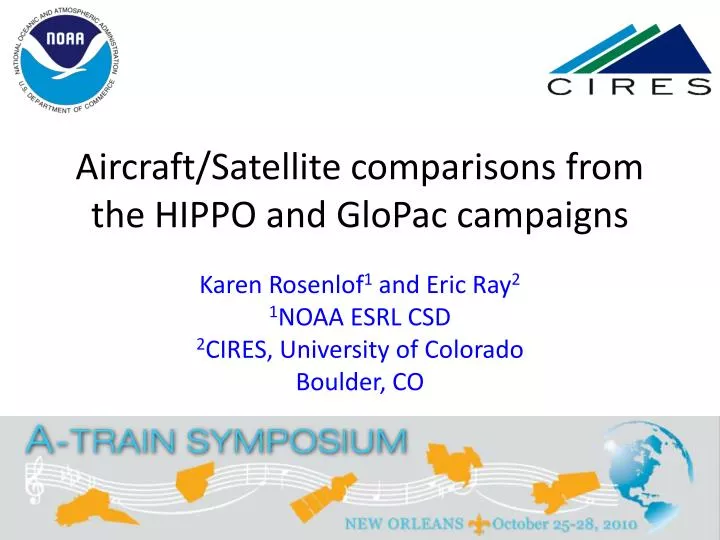
Aircraft/Satellite comparisons from the HIPPO and GloPac campaigns Karen Rosenlof1 and Eric Ray2 1NOAA ESRL CSD 2CIRES, University of Colorado Boulder, CO
HIAPER Pole-to-Pole Observations (HIPPO) • What is HIPPO? • High resolutions measurements over the entire latitude range of the Pacific • Uses the NCAR Gulfstream-V • Multi-deployment experiment • Emphasis on carbon cycle and greenhouse gases • 3 deployments are complete, data is finalized from HIPPO1 and nearly so for HIPPO2 • There will be 2 additional deployments in 2011 • This is the first comprehensive aircraft based global survey of trace gases pertinent to the carbon cycle covering the full depth of the troposphere in all seasons and multiple years
The HIPPO data set is intended to provide critical tests of global models of atmospheric gases and aerosols, helping to distinguish errors associated with sources and sinks from those due to simulated transport, model structure, etc. The NCAR Gulfstream V has a ceiling of ~ 51kFt, a range of 7000 miles. payload capacity of 5600 lbs At PANC during HIPPO I, Jan 2009
HIPPO Instrumentation Multiple measurements:Red symbols≥ 3, Blue = 2; sampling rates in ().
HIPPO Scientific Team: Steve Wofsy: Principal Investigator, Harvard University Britt Stephens: Co-PI, Airborne Oxygen instrument and MEDUSA air sampler, NCAR Ralph Keeling: Co-PI, MEDUSA air sampler, Scripps Bruce Daube: Mission Scientist / Instrumentation Engineer, Harvard University Jasna Pittman, RoisinCommane, Bin Xiang, Eric Kort: QCLS and CO2 instruments, Harvard University Elliot Atlas: Whole Air Sampler, University of Miami James Elkins, Steve Montzka (NOAA) Fred Moore, David Nance, Eric Hintsa (CU CIRES): PANTHER, NOAAWAS and UCATS instruments Jonathan Bent, Steve Shertz: MEDUSA and AO2 Instruments, Scripps David Fahey, Ru-Shan Gao: Ozone / SP2 instruments, NOAA Christopher Picket-Heaps: chemical modeling, Harvard University Eric Ray (CIRES), Karen Rosenlof (NOAA): flight forecasting Shuka Schwarz, Ryan Spackman, Laurel Watts, Steve Ciciora, Anne Perring: NOAA Ozone and SP2 instruments, CU CIRES Mark Zondlo: VCSEL instrument, Princeton University Teresa Campos: CO instrument, NCAR Julie Haggerty: MTP, NCAR M.J. Mahoney: MTP, JPL NCAR RAF: Aircraft support, project management, data catalog management
HIPPO Statistics 2009 201020082011 20112009 H1 H3 P-H H4 H5 H2 Day of Year To Date: 156 days of field program, 524 profiles National Science Foundation National Oceanic and Atmospheric Administration G-V "HIAPER": National Center for Atmospheric Research HIPPO Sponsors
HIPPO itinerary HIPPO_2 Nov 2009 START08/preHIPPO Apr-Jun 2008 HIPPO_3 Apr 2010 HIPPO_1 Jan 2009
Example of vertical coverage: shows there is some coverage in the lower stratosphere (noted in blue below), so potentially useful for some MLS comparisons.
Although the main intent for use of this set of data is in regards to understanding processes and model comparisons/validations, it is also useful for satellite measurement comparisons. HIPPO flights were not planned with satellite validation in mind. We had specific destinations predetermined, and what small deviations from great circle routes that were possible were geared to sampling specific features ascertained from chemical forecast models and current satellite observations. However, in the case of AIRS coverage is sufficiently dense that coincidences on the day of a flight were fairly common. We did have one flight day that was designed to be along an Aura track and was also coincident with the ground track of the NASA Global-Hawk. For this case, MLS comparisons are also possible.
HIPPO-1 Atmospheric Structure (Pot'l T K): January, 2009, Mid-Pacific (Dateline) Cross section
HIPPO sections, January 2009 CO CO2 CH4 0 5 10 15 km 0 5 10 15 km 0 5 10 15 km -60 -40 -20 0 20 40 60 80 -60 -40 -20 0 20 40 60 80 -60 -40 -20 0 20 40 60 80 N2O SF6 O3 0 5 10 15 km 0 5 10 15 km 0 5 10 15 km -60 -40 -20 0 20 40 60 80 -60 -40 -20 0 20 40 60 80 -60 -40 -20 0 20 40 60 80 LATITUDE
Species we have done HIPPO/AIRS comparisons with are: O3 H2O CO CH4 CO2 Temperature HIPPO measurements may also be useful for satellite aerosol comparisons (Ryan Spackman had a poster discussing possible use of HIPPO black carbon measurements for satellite validation.) A unique feature about HIPPO that satellite groups may find useful: There are many profiles in the Southern Hemisphere, covering a region that has not been heavily sampled by recent aircraft experiments. There are ~140 profiles from the surface to 8 km, and ~20 from the surface to max altitude on each deployment. (3 deployments to date, 5 in total by the end of FY11. Although we looked exclusively at AIRS comparisons, these measurements could also be useful for TES and IASI comparisons, or any instrument measuring tropospheric ozone profiles. Could also be used for comparisons with high latitude lower stratospheric measurements.
Global Hawk coordinated flights and satellite validation Anchorage GloPac GH track HIPPO NSF/NCAR GV J. Schwarz Aura satellite track follows the western side of the GloPac flight. 70 mb Ozone field from Aura Microwave Limb Sounder (MLS). Hawaii 13 April 2010
Comparison of Global Hawk and NSF/NCAR GV correlations of CH4 with N2O Coordinated flights allow unique sampling of tracer space in UT/LS Overflight segment Tropopause range All data Overflight segment data only Increasing altitude and age-of-air Preliminary data: QCLS, Wofsy et al.; UCATS, Hintsa et al.
What could be possible with these two platforms? Coordinated flights allow unique sampling of tracer space in UT/LS Tropopause range If appropriately coordinated, between the two platforms can get vertical profiles through the UTLS at all latitudes, then would be able to apply satellite weighting functions. With the G-Hawk based in California with a 30 hour duration, and the G-V flying between multiple bases, it would be possible to cover a large portion of the NH Pacific.
Final Notes: HIPPO provides fine resolution data covering the latitudinal extent of the Pacific for a number of species. There are approximately 140 profiles per deployment, with 3 deployments completed, and 2 more planned. HIPPO 1 data is finalized, should be publically available soon. An initial publication (Wofsy et al.) will appear in the near future (Royal Society proceedings) Official data archive will be at the CDIAC (ornl.gov); data is currently at an NCAR mission data catalog site.
AIRS-HIPPO Comparison Method Small circles represent fine layers in example trapezoid HIPPO data within 50 km of example AIRS profile • Identify nearest AIRS profiles to HIPPO flight tracks (≈2500 for 3 missions). • For each AIRS profile find HIPPO measurements within 50 km and 6 hours. • For AIRS layer quantities we divide the layer into 10-20 finer layers and the layer difference is: • where z is the fine layer where HIPPO data is available and W is the layer weighting function. • For CO2, we simply took a 2-8 km profile average, and found the AIRS profile closest in space on a given flight day.