Download
1 / 53
530 likes | 706 Views
UCLA NS 172/272/Psych 213 Brain Mapping and Neuroimaging. Instructor : Ivo Dinov , Asst. Prof. In Statistics and Neurology University of California, Los Angeles, Winter 2006 http://www.stat.ucla.edu/~dinov/ http://www.loni.ucla.edu/CCB/Training/Courses/NS172_2006.shtml.

E N D
UCLA NS 172/272/Psych 213Brain Mapping and Neuroimaging Instructor: Ivo Dinov, Asst. Prof. In Statistics and Neurology University of California, Los Angeles, Winter 2006 http://www.stat.ucla.edu/~dinov/ http://www.loni.ucla.edu/CCB/Training/Courses/NS172_2006.shtml
References • “Foundation of Medical Imaging,” Z.H. Cho, J.P. Jones, M. Singh, John Wiley & Sons, Inc., New York 1993, ISBN 0-471-54573-2 • “Principles of Medical Imaging,” K.K. Shung, M.B. Smith, B. Tsui, Academic Press, San Diego 1992, ISBN 0-12-640970-6 • “Handbook of Medical Imaging,” Vol. 1, Physics and Psychophysics, J. Beutel, H. L. Kundel, R. L. Van Metter (eds.), SPIE Press 2000, ISBN 0-8194-3621-6 • Brain Mapping: The Methods, by Arthur W. Toga & John Mazziotta
Introduction: What is Medical Imaging? • Goals: • Create images of the interior of the living human body from the outside for diagnostic purposes. • Biomedical Imaging is a multi-disciplinary field involving • Physics (matter, energy, radiation, etc.) • Math (linear algebra, calculus, statistics) • Biology/Physiology • Engineering (implementation) • Computer science (image reconstruction, signal processing, visualization)
BMI methods: X-Ray imaging • Year discovered: 1895 (Röntgen, NP 1905) • Form of radiation: X-rays = electromagnetic radiation (photons) • Energy / wavelength of radiation: 0.1 – 100 keV / 10 – 0.01 nm (ionizing) • Imaging principle: X-rays penetrate tissue and create shadowgram of differences in density. • Imaging volume: Whole body • Resolution: Very high (sub-mm) • Applications: Mammography, lung diseases, orthopedics, dentistry, cardiovascular, GI, neuro
Radio wave devices AM radio - 535 kilohertz to 1.7 megahertz [Frequency ~ 106] Short wave radio - bands from 5.9 megahertz to 26.1 megahertz Citizens band (CB) radio - 26.96 megahertz to 27.41 megahertz Television stations - 54 to 88 megahertz for channels 2 through 6 FM radio - 88 megahertz to 108 megahertz Television stations - 174 to 220 megahertz
BMI methods: X-Ray Computed Tomography • Year discovered: 1972 (Hounsfield, NP 1979) • Form of radiation: X-rays • Energy / wavelength of radiation: 10 – 100 keV / 0.1 – 0.01 nm (ionizing) • Imaging principle: X-ray images are taken under many angles from which tomographic ("sliced") views are computed • Imaging volume: Whole body • Resolution: High (mm) • Applications: Soft tissue imaging (brain, cardiovascular, GI)
BMI methods: Nuclear Imaging (PET/SPECT) • Year discovered: 1953 (PET), 1963 (SPECT) • Form of radiation: Gamma rays • Energy / wavelength of radiation: > 100 keV / < 0.01 nm (ionizing) • Imaging principle: Accumulation or "washout" of radioactive isotopes in the body are imaged with x-ray cameras. • Imaging volume: Whole body • Resolution: Medium – Low (mm - cm) • Applications: Functional imaging (cancer detection, metabolic processes, myocardial infarction)
Functional Brain Imaging - Positron Emission Tomography (PET)
Functional Brain Imaging - Positron Emission Tomography (PET) http://www.nucmed.buffalo.edu
Functional Brain Imaging - Positron Emission Tomography (PET) Isotope Energy (MeV) Range(mm) 1/2-life Appl’n C 0.96 1.1 20 min receptor studies O 1.7 1.5 2 min stroke/activation F 0.64 1.0 110 min neurology I ~2.0 1.6 4.5 days oncology 11 15 18 124 E:\Ivo.dir\LONI_Viz\LOVE_Distribution_062105\runNoArgs.bat Load Volumes: E:\Ivo.dir\LONI_Viz\data.dir\A1_Global.img E:\Ivo.dir\LONI_Viz\data.dir\R12_Global.img Subsample 2-2-2 VolumeRenderer + 2D Section + Change ColorMap
BMI methods: Magnetic Resonance Imaging • Year discovered: 1945 (Bloch & Purcell) 1973 (Lauterburg, NP 2003) 1977 (Mansfield, NP 2003) 1971 (Damadian, SUNY DMS) • Form of radiation: Radio frequency (RF) (non-ionizing) • Energy / wavelength of radiation: 10 – 100 MHz / 30 – 3 m (~ 10-7 eV) • Imaging principle: Proton spin flips are induced, and the RF emitted by their response (echo) is detected. • Imaging volume: Whole body • Resolution: High (mm) • Applications: Soft tissue, functional imaging
BMI methods: Ultrasound Imaging • Year discovered: 1952 (Norris, clinical: 1962) • Form of radiation: Sound waves (non-ionizing) • Frequency / wavelength of radiation: 1 – 10 MHz / 1 – 0.1 mm • Imaging principle: Echoes from discontinuities in tissue density/speed of sound are registered. • Imaging volume: < 20 cm • Resolution: High (mm) • Applications: Soft tissue, blood flow (Doppler)
BMI methods: Optical Tomography • Year discovered: 1989 (Barbour) • Form of radiation: Near-infrared light (non-ionizing) • Energy / wavelength of radiation: ~ 1 eV/ 600 – 1000 nm • Imaging principle: Interaction (absorption, scattering) of light w/ tissue. • Imaging volume: ~ 10 cm • Resolution: Low (~ cm) • Applications: Perfusion, functional imaging
Recipe for MRI • 1) Put subject in big magnetic field (leave him/her there) • 2) Transmit radio waves into subject [about 3 ms] • 3) Turn off radio wave transmitter • 4) Receive radio waves re-transmitted by subject • Manipulate re-transmission with magnetic fields during this readout interval [10-100 ms: MRI is not a snapshot] • 5) Store measured radio wave data vs. time • Now go back to 2) to get some more data • 6) Process raw data to reconstruct images • 7) Allow subject to leave scanner • Example of non-homogeneity effects in MRI: • E:\Ivo.dir\LONI_Viz\LOVE_Distribution_062105\runNoArgs.bat E:\Ivo.dir\Research\Data.dir\LianaApostolova_AD\FrontalVolumes2Groups/MRI_ToothMetal_Defect.img.gz • E:\Ivo.dir\LONI_Viz\LONI_Viz_VR_MetalToothDefect.bat Source: Robert Cox’s web slides
most likely explanation: nuclear has bad connotations less likely but more amusing explanation: subjects got nervous when fast-talking doctors suggested an NMR History of NMR • NMR = nuclear magnetic resonance • Felix Block and Edward Purcell • 1946: atomic nuclei absorb and re-emit radio frequency energy • 1952: Nobel prize in physics • nuclear: properties of nuclei of atoms • magnetic: magnetic field required • resonance: interaction between magnetic field and radio frequency Bloch Purcell NMR MRI: Why the name change?
Ogawa History of fMRI MRI -1971: MRI Tumor detection (Damadian) -1973: Lauterbur suggests NMR could be used to form images -1977: clinical MRI scanner patented -1977: Mansfield proposes echo-planar imaging (EPI) to acquire images faster fMRI -1990: Ogawa observes BOLD effect with T2* blood vessels became more visible as blood oxygen decreased -1991: Belliveau observes first functional images using a contrast agent -1992: Ogawa et al. and Kwong et al. publish first functional images using BOLD signal
Magnet Gradient Coil RF Coil Necessary Equipment 4T magnet RF Coil gradient coil (inside) Source: Joe Gati, photos
Robarts Research Institute 4T B0 x 80,000 = The Big Magnet • Very strong • 1 Tesla (T) = 10,000 Gauss • Earth’s magnetic field = 0.5 Gauss • 4 Tesla = 4 x 10,000 0.5 = 80,000 times Earth’s magnetic field • Continuously on • Main field = B0
Source: www.howstuffworks.com Source: http://www.simplyphysics.com/ flying_objects.html Magnet Safety - The whopping strength of the magnet makes safety essential. Things fly – Even big things! Screen subjects carefully Make sure you and all your students & staff are aware of hazards Develop strategies for screening yourself every time you enter the magnet
Subject Safety • Anyone going near the magnet – subjects, staff and visitors – must be thoroughly screened: • Subjects must have no metal in their bodies: • pacemaker • aneurysm clips • metal implants (e.g., cochlear implants) • interuterine devices (IUDs) • some dental work (fillings okay) • Subjects must remove metal from their bodies • jewellery, watch, piercings • coins, etc. • wallet • any metal that may distort the field (e.g., underwire bra) • Subjects must be given ear plugs (acoustic noise can reach 120 dB) • C:\Ivo.dir\Research\Data.dir\LianaApostolova_AD\FrontalVolumes2Groups\MRI_ToothMetal_Defect.img.gz (Show-VolumeRenderer) • C:\Ivo.dir\LONI_Viz\LONI_Viz_MAP_demo\runNoArgs.bat This subject was wearing a hair band with a ~2 mm copper clamp. Left: with hair band. Right: without. Source: Jorge Jovicich
Protons • Can measure nuclei with odd number of neutrons • 1H, 13C, 19F, 23Na, 31P • 1H (proton) - Human body 70+% H2O • abundant: high concentration in human body high sensitivity: yields large signals Both protons and neutrons possess spins, i.e. they revolve round their own axis, much as earth does. If the nucleus has just one proton, it would spin on its axis and would impart a net spin to the nucleus as a whole. One would imagine that two protons would double up the spin for the nucleus but it doesn’t happen that way; the spins of the two protons tend to cancel out, with the result that the nucleus has no net spin. A nucleus with three protons again has a net spin (as there is one unpaired proton) and a nucleus with four protons again would have no spin. The same is true for neutrons; an odd number of neutrons imparts a net spin to the nucleus, an even number doesn’t. So out of protons or neutrons if any one of these (or both) are in odd number, the nucleus would have a net spin. If both are even, the nucleus would not have any net spin.
What nuclei exhibit this magnetic moment (and thus are candidates for NMR)? Nuclei with: odd number of protons odd number of neutrons odd number of both Magnetic moments: 1H, 2H, 3He, 31P, 23Na, 17O, 13C, 19F No magnetic moment: 4He, 16O, 12C
Source: Mark Cohen’s web slides Source: Robert Cox’s web slides Outside magnetic field – random orientationIn Mag Field - Protons align with field • randomly oriented Inside magnetic field • spins tend to align parallel or anti-parallel to B0 • net magnetization (M) along B0 • spins precess with random phase • no net magnetization in transverse plane • only 0.0003% of protons/T align with field M longitudinal axis Longitudinal magnetization transverse plane M = 0
Radio Frequency As its name implies, NMR is a resonance phenomenon. This means that it will occur only if the applied RF pulse is tuned to the natural resonance frequency of the nucleus in question. The natural resonance frequency of any given nucleus depends on the strength of the applied main magnetic field; more strength higher frequency. 4T fMRI Broadcasts at a frequency of 170.3 MHz! To locate each atom within the sample make the main magnetic field graded so that it is not of uniform strength but rather increases slightly in strength from one side of the sample to the other, the resonance frequencies of different nuclei would differ.
170.3 Resonance Frequency for 1H 63.8 1.5 4.0 Field Strength (Tesla) Larmor Frequency Larmor equation (frequency) f = B0 (field strength) = 42.58 MHz/T (constant for each Atom). For example for Hydrogen: At 1.5T, f = 63.76 MHz At 4T, f= 170.3 MHz
B0 B1 RF Excitation • Excite Radio Frequency (RF) field • transmission coil: apply magnetic field along B1 (^ to B0) for ~3 ms • oscillating field at Larmor frequency • frequencies in range of radio transmissions • B1 is small: ~1/10,000 T • tips M to transverse plane – spirals down • analogies: guitar string, swing • final angle between B0 and B1 is the flip angle Transverse magnetization Source: Robert Cox’s web slides
Relaxation and Receiving • Receive Radio Frequency Field • receiving coil: measure net magnetization (M) • readout interval (~10-100 ms) • relaxation: after RF field turned on and off, magnetization returns to normal • longitudinal magnetization T1 signal recovers • transverse magnetization T2 signal decays Source: Robert Cox’s web slides
T1 and TR • T1 = recovery of longitudinal (B0) magnetization • used in anatomical images • ~500-1000 msec (longer with bigger B0) • TR (repetition time) = time to wait after excitation before sampling T1 Source: Mark Cohen’s web slides
excite only frequencies corresponding to slice plane Freq Field Strength (T) ~ z position Gradient coil Spatial Coding: Gradients • How can we encode spatial position? • Example: axial slice Add a gradient to the main magnetic field • Use other tricks to get other two dimensions • left-right: frequency encode • top-bottom: phase encode Gradient switching – that’s what makes all the beeping & buzzing noises during imaging!
How many fields are involved after all? In MRI there are 3 kinds of magnetic fields: 1. B0 – the main magnetic field 2. B1 – an RF field that excites the spins 3. Gx, Gy, Gz – the gradient fields that provide localization
Precession In and Out of Phase • Protons precess at slightly different frequencies because of • random fluctuations in local field at the molecular level affect both T2 and T2*; (2) larger scale variations in the magnetic field (such as the presence of deoxyhemoglobin!) that affect T2* only. • Over time, the frequency differences lead to different phases between the molecules (think of a bunch of clocks running at different rates – at first they are synchronized, but over time, they get more out of sync until they are random) • As the protons get out of phase, the transverse magnetization decays • This decay occurs at different rates in different tissues Source: Mark Cohen’s web slides
T2 and TE T1 = recovery of longitudinal (B0) magnetization TR (repetition time) = time to wait after excitation before sampling T1 T2 = decay of transverse magnetization TE (time to echo) = time to wait to measure T2 or T2* (after refocussing with spin echo or gradient echo) Source: Mark Cohen’s web slides
Echos Pulse sequence: series of excitations, gradient triggers and readouts Gradient echo pulse sequence Echos – refocussing of signal Spin echo – use a 180 degree pulse to “mirror image” the spins in the transverse plane when “fast” regions get ahead in phase, make them go to the back and catch up • measure T2 • ideally TE = average T2 • Gradient echo – flip the gradient from negative to positive make “fast” regions become “slow” and vice-versa • measure T2* • ideally TE ~ average T2* t = TE/2 A gradient reversal (shown) or 180 pulse (not shown) at this point will lead to a recovery of transverse magnetization TE = Time to Echo – wait to measure refocussed spins Source: Mark Cohen’s web slides
T1 vs. T2 Repetition Time: Time to Echo Source: Mark Cohen’s web slides
T1 vs. T2 – contrast and noise Source: Mark Cohen’s web slides
Tissue T1 (ms) T2 (ms) Grey Matter (GM) 950 100 White Matter (WM) 600 80 Muscle 900 50 Cerebrospinal Fluid (CSF) 4500 2200 Fat 250 60 Blood 1200 100-200 Properties of Body Tissues MRI has high contrast for different tissue types!
MRI of the Brain - Sagittal T1 Contrast TE = 14 ms TR = 400 ms T2 Contrast TE = 100 ms TR = 1500 ms Proton Density TE = 14 ms TR = 1500 ms
MRI of the Brain - Axial T1 Contrast TE = 14 ms TR = 400 ms T2 Contrast TE = 100 ms TR = 1500 ms Proton Density TE = 14 ms TR = 1500 ms
Relative SNR Field of View MRI Quality Determinants • Echo Time (TE) • Slice Thickness • Slice Order • Averaging • Bandwidth • Imaging Matrix • Patient Motion • Surface Coils • Repetition Time(TR) • Interslice Gap • Field of View • Number of Echos • Motion Comp • Window Level • Photography • Equipment Performance • Mark Cohen
K-Space – an MRI literaturefancy name for Fourier space Source: Traveler’s Guide to K-space (C.A. Mistretta) http://www.cis.rit.edu/htbooks/mri/
both halves of k-space in 1 sec 1st half of k-space in 0.5 sec 2nd half of k-space in 0.5 sec 1st half of k-space in 0.5 sec 2nd half of k-space in 0.5 sec interpolated image 2nd volume in 1 sec A Walk Through (sampling from ) K-space single shot two shot • K-space can be sampled in many “shots” • (or even in a spiral) • 2 shot or 4 shot • less time between samples of slices • allows temporal interpolation Note: The above is k-space, not slices vs. 1st volume in 1 sec
Mxy Mo sin T2 T2* time T2* • T2* relaxation - Sequences without a spin echo will be T2*-weighted rather than T2-weighted. The longer the echo time (TE) the greater the T2 contrast. • - dephasing of transverse magnetization due to both: • - microscopic molecular interactions (T2) • - spatial variations of the external main field B • (tissue/air, tissue/bone interfaces) • exponential decay (T2* 30 - 100 ms, shorter for higher Bo) Source: Jorge Jovicich