Download
1 / 15
150 likes | 257 Views
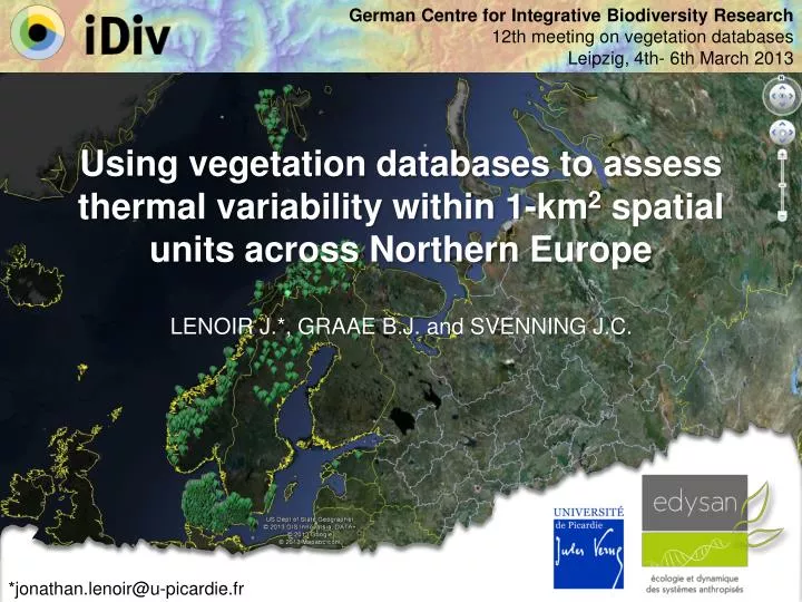
German Centre for Integrative Biodiversity Research 12th meeting on vegetation databases Leipzig , 4th- 6th March 2013. Using vegetation databases to assess thermal variability within 1-km 2 spatial units across Northern Europe LENOIR J.*, GRAAE B.J. and SVENNING J.C.

E N D
German Centre for Integrative Biodiversity Research 12th meeting on vegetation databases Leipzig, 4th- 6th March 2013 Using vegetation databases to assess thermal variability within 1-km2 spatial units across Northern Europe LENOIR J.*, GRAAE B.J. and SVENNING J.C. *jonathan.lenoir@u-picardie.fr
Why caring about fine-grained thermal variability? Furka pass in the Swiss Alps: Using high-resolution thermal imaging, Scherrer and Körner (2010) have shown that mean temperature during day time can range from 6 to 24C within this small area (b) Night temperatures Day temperatures Ccl: Short-distance escapes are available for plants to persist locally amidst unfavorable regional climatic conditions suggesting plant biodiversity to be less endangered than is expected by climate warming projections Introduction Materials Methods Results Conclusions
How big is this thermal variability at broad scales? • Issue: • This information is not yet available because the cost of using data loggers or high-resolution thermal imaging across large spatial extents is a limiting factor • Solution: • Vegetation geodatabasesare already available across large spatial extents and can be used in combination with semi-quantitative plant species indicator values to infer biologically relevant temperature conditions from plant assemblages within <1000-m2units (community-inferred temperatures: CiT) Introduction Materials Methods Results Conclusions
Main questions and objectives • Assessing thermal variability (CiT range) within 1-km2 units (cf. WorldClim climatic unit, http://www.worldclim.org/) • Analyzing the relationship between CiT range and variables reflecting terrain complexity (elevation range, roughness, etc.) at 1-km resolution • Testing whether or not spatial turnover in CiT is greater than spatial turnover in globally interpolated temperatures (cf. WorldClimtemperature grids) ? ΔCiT(C) CiT range (C) 1 km 1 km Elevation range (m) ? CiT Δ global T (C) CiT range? Distance (m) Introduction Materials Methods Results Conclusions
Plot-scale data • 42117 vegetation plots across Northern Europe • 138 of these plots are equipped with miniature soil data-loggers MAT (°C) Elevation (m) Introduction Materials Methods Results Conclusions
Gridded data • 1 digital elevation model grid across Northern Europe at 33-m resolution (ASTERGDEM) • 12 mean monthly temperature grids across Northern Europe at 1-km resolution (WorldClim) (m) Dec (MMT12) Nov (MMT11) (°C) Oct (MMT10) 1 km Sep (MMT9) Aug (MMT8) Jul (MMT7) Jun (MMT6) May (MMT5) Apr (MMT4) Mar (MMT3) For each 1-km2 unit, we computed: eleR, slopR, northR, eastR, expoRand roughM Feb (MMT2) Jan (MMT1) Introduction Materials Methods Results Conclusions
Bottom-up modeling approach to compute CiT 1-km2spatial unit (m) Ellenberg averaged value: EaV (T) = 3 MMT7 from data-logger: LmT = -1°C LmT (°C) MMT7 MMT7 LmT (°C) CiT = -4°C 138 vegetation plots Ellenberg averaged value, EaV (T) Ellenberg averaged value, EaV (T) Introduction Materials Methods Results Conclusions
Top-down modeling approach to compute CiT (°C) 1-km2spatial unit Ell. (T) Ellenberg averaged value: EaV (T) = 3 MMT7 from WorldClim: GiT = -1°C GiT (°C) MMT7 MMT7 GiT (°C) CiT = -4°C 121 1-km2 units 1-km2-mean EaV (T) 1-km2-mean EaV(T) Introduction Materials Methods Results Conclusions
CiT reflects mean growing-season temperature June, July, August Calibration Validation Bottom-up approach Top-down approach J J F F M M A A M M J J J J A A S S O O N N D D Introduction Materials Methods Results Conclusions
1-km2 thermal variability ranges from 0 to 7°C • 569 1-km2WorlClim units used to assess thermal variability across Northern Europe • Thermal variability averages 2.1°C (SD = 0.97°C) across Northern Europe Introduction Materials Methods Results Conclusions
Rough terrains offer high thermal variability • Thermal variability peaks at 60–65°N, where rough terrains are predominant due to the gross topography from southern to mid-Norway • Thermal variability increases with terrain roughness averaging 1.97°C (SD = 0.84°C) and 2.68°C (SD = 1.26°C) within the flattest (PC1 < 0) and roughest (PC1 > 0) 1-km2WorldClimunits respectively Elevation range (m) Introduction Materials Methods Results Conclusions
Thermal variability increases spatial turnover • 349 100-km2WorldClimunits used to assess spatial turnover in community-inferred temperature (CiT) and globally interpolated temperature (GiT) • Spatial turnover in CiT within 100-km2 units was, on average, 1.8 times greater (0.32°C/km) than spatial turnover in GiT (0.18 °C/km) Introduction Materials Methods Results Conclusions
Take-home messages • Fine-grained (1 km2) thermal variability increases local spatial buffering of future climate warming, even in the flattest terrains, and may provide short-distance escapes for species to persist locally amidst unfavorable regional climatic conditions • Coarse-scale species distribution models ignoring this thermal variability tend to overestimate future species’ range shifts and future biodiversity loss • Our community-based approach may better reflects temperature conditions biologically relevant to plant community dynamics than measurements from short-term, localized miniature soil data-loggers even though it underestimated the actual fine-grained thermal variability Introduction Materials Methods Results Conclusions
For more information Introduction Materials Methods Results Conclusions
German Centre for Integrative Biodiversity Research 12th meeting on vegetation databases Leipzig, 4th- 6th March 2013 Acknowledgements - The Stay Or Go Network (http://www.ntnu.edu/stay-or-go/) - All my co-authors for their active contribution to this work - The many people who collected the field data - David Ackerly for insightful comments - Ute Jandt & HelgeBruelheide for organizing this meeting - And all of you for your attention *jonathan.lenoir@u-picardie.fr