Download
1 / 39
390 likes | 569 Views
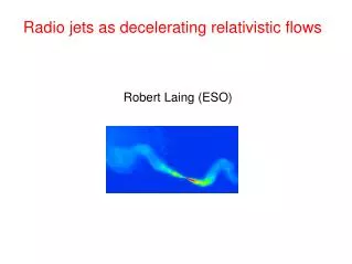
Radio jets as decelerating relativistic flows. Robert Laing (ESO). A weak (FRI) radio galaxy. Tail. Tail. Jets. 3C 31 (VLA 1.4GHz; 5.5 arcsec FWHM). Jets in FRI sources decelerate, becoming trans- or subsonic and produce much of their radiation close to the nucleus. FRII radio galaxy.

E N D
Radio jets as decelerating relativistic flows Robert Laing (ESO)
A weak (FRI) radio galaxy Tail Tail Jets 3C 31 (VLA 1.4GHz; 5.5 arcsec FWHM) Jets in FRI sources decelerate, becoming trans- or subsonic and produce much of their radiation close to the nucleus
FRII radio galaxy 3C 353 (VLA, 8.4 GHz, 0.44 arcsec) FRII jets remain supersonic (and relativistic) until the hot-spots
Modelling of FRI jets • Model FRI jets as intrinsically symmetrical, axisymmetric, relativistic flows [free models]. Derive 3D velocity, emissivity and field geometry. [Deep, high-resolution radio images. Linear polarization essential.] • Apply conservation of mass, momentum and energy to infer the variations of pressure, density, entrainment rate and Mach number. [External density and pressure from X-ray observations.] • Model the acceleration and energy-loss processes, starting with adiabatic models. [Images at mm, IR, optical, X-ray wavelengths.]
Progress so far • B2 sample statistics (Laing et al. 1999) • Free models of 3C31 (Laing & Bridle 2002a) • Conservation-law analysis of 3C 31 (Laing & Bridle 2002b) • Adiabatic models of 3C 31 (Laing & Bridle 2004) • Free models of B2 0326+39 and 1553+24 (Canvin & Laing 2004) • Free model of NGC 315 (Canvin et al., MNRAS, nearly) Alan Bridle, James Canvin – models Diana Worrall, Martin Hardcastle, Mark Birkinshaw (Bristol UH) – X-ray Bill Cotton, Paola Parma, Gabriele Giovannini, … - radio
Free models – basic principles • Model jets as intrinsically symmetrical, axisymmetric, relativistic, stationary flows. Fields are disordered, but anisotropic (see later) • Parameterize geometry, velocity, emissivity and field structure. • Optimize model parameters by fitting to IQU images. • Derive model IQU by integration along the line of sight, taking account of anisotropy of synchrotron emission in the rest frame, aberration and beaming. • Linear polarization is essential to break the degeneracy between angle and velocity.
Degree of polarization B2 1553+24 NGC 315 3C 31 B2 0326+29 Correlated asymmetry between I sidedness and polarization
Breaking the β – θ degeneracy • For isotropic emission in the rest frame, jet/counter-jet ratio depends on βcosθ – how to separate? • But B is not isotropic, so rest-frame emission (IQU) depends on angle to line of sight in that frame θ′ • sin θ′ = D sin θ and D = [Γ(1± βcosθ)]-1 is different for the main and counter-jets • So the polarization is different for the two jets • If we knew the field, we could separate β and θ • We don’t, but we can fit the transverse variation of polarization and determine field component ratios • Need good transverse resolution and polarization
Total Intensity θ 8o 37o 52o 64o B2 1553+24 NGC 315 3C 31 B2 0326+39
Total Intensity (high resolution) θ = 8o 37o 52o 64o
Degree of polarization θ 8o 37o 52o 64o
Apparent magnetic field (1) θ = 8o 37o
Apparent magnetic field (2) θ = 52o 64o
Velocity β = v/c B2 1553+24 NGC 315 B2 0326+39 3C 31
Velocity, spines and shear layers • β≈ 0.8-0.9 where the jets first brighten • All of the jets decelerate abruptly in the flaring region, but at different distances from the nucleus. • At larger distances, three have roughly constant velocities in the range β≈ 0.1 – 0.4 and one (3C 31) decelerates slowly • They have transverse velocity gradients, with edge/on-axis velocity consistent with 0.7 everywhere. • No obvious low-velocity wings. • No large differences in Γ or narrow shear layers • We no longer favour a separate spine – transverse profiles are as well fit by a single truncated Gaussian (but see next slide) • Large uncertainties where jets are slow or poorly resolved
Transverse velocity profile may be more complex NGC 315 (best resolved case) Full line = measured sidedness ratio Dashed = model (truncated Gaussian velocity profile) Shear at intermediate radii?
Helical Fields? θ = 45o θ = 90o Synchrotron emission from a helical field with pitch angle 45o
Helical Fields? • Helical fields generally produce brightness • and polarization distributions which have • asymmetric transverse profiles • The profiles are symmetrical only if: • there is no longitudinal component or • the jet is at 90o to the line of sight in the • rest frame of the emitting material • The condition for the approaching jet to • be observed side-on in the rest frame is • β = cosθ - also the condition for maximum • Doppler boost: hence a selection effect in • favour for blazar jets • Never true in counter-jet unless β = 0 or • θ = 90o
Helical Fields in FRI jets? Transverse profiles of I and p for NGC315 – symmetrical, especially in counter-jet Not a helical field (but could be ordered toroidal + longitudinal with reversals)
Helical Fields in FRII jets? 3C353 (Swain, Bridle & Baum 1998) Profiles are very symmetrical – field probably not helical
Field component evolution in NGC 315 Radial Longitudinal Toroidal
Field structure • Fields on kpc scales are not vector-ordered helices. Nor should they be (poloidal flux proportional to r-2) • Transverse (i.e. radial+toroidal) field spine + longitudinal-field shear layer predicts field transition closer to the nucleus in the main jet – not observed. • Field is primarily toroidal + longitudinal, with smaller radial component. • Toroidal component could be ordered, provided that the longitudinal field has many reversals.
Digression: rotation measure gradients 3C 31 Rotation measure Counter-jet Main jet Total intensity
Linearity of χ – λ2 relation Linearity of χ - λ2 relation and very small depolarization requires foreground Faraday rotation
Modelling RM variations Realisation of a random magnetic field with a power-law energy spectrum in the group gas associated with 3C 31 RM calculated for a plane at 52o to the line of sight, as for the jet model (near side on the right)
Emissivity and field • Emissivity profile tends to flatten at large distances from the nucleus (compare with adiabatic models – later). • FRI jets are intrinsically centre-brightened. • Dominant field component at large distances is toroidal. • The longitudinal component can be significant close to the nucleus, but decreases further out. • Radial component behaviour is peculiar. • Qualitatively consistent with flux freezing, but laminar-flow models, even including shear, do not fit.
Conservation law analysis • We now know the velocity and area of the jet. • The external density and pressure come from Chandra observations. • Solve for conservation of momentum, matter and energy. • Include buoyancy • Well-constrained solutions exist. • Key assumptions: Energy flux = momentum flux x c Pressure balance in outer region
Conservation-law analysis: fiducial numbers at the jet flaring point • Mass flux 3 x 10¹⁹ kgs-1 (0.0005 solar masses/yr) • Energy flux 1.1 x 1037 W • Pressure 1.5 x 10⁻¹⁰ Pa • Density 2 x 10-27 kgm-3 • Mach number 1.5 • Entrainment rate 1.2 x 10¹⁰ kgkpc-1s-1
Presssure, density, Mach number, entrainment Mach number (transonic) Entrainment rate Pressure Density
What are the jets made of? • r = 2.3 x 10⁻²⁷ kg m-3 (equivalent to 1.4 protons m-3) at the flaring point. • For a power-law energy distribution of radiating electrons, n = 60 gmin-1.1 m-3 (~10-28 gmin-1.1 kg m-3). • Possibilities include: • Pure e+e- plasma with an excess of particles over a power law at low energies. • e+e- plasma with a small amount of thermal plasma. • Cold protons in equal numbers with radiating electrons and gmin = 20 - 50 (not observable).
Adiabatic models Set initial conditions at start of outer region. Calculate evolution of particle density and field assuming adiabatic/flux- freezing in a laminar flow. Adiabatic models give a reasonable fit, but do not get either the intensity or polarization quite right. Not surprising if the flow is turbulent?
Adiabatic models 3C 31 I Free model Adiabatic, with same velocity Adiabatic model with distributed and initial conditions. particle injection.
Where are particles injected? Points – X-ray Full line – particle injection function Dashed line - radio VLA + Chandra Internal p Pressures from conservation-law analysis External p Minimum p
Changing the angle to the line of sight: Unified models
Conclusions • FRI jets are decelerating relativistic flows, which we can now model quantitatively. • The 3D distributions of velocity, emissivity and field ordering can be inferred by fitting to radio images in total intensity and linear polarization. • Application of conservation of energy and momentum allows us to deduce the variation of density, pressure and entrainment rate along the jet. • Boundary layer entrainment and mass input from stars are probably both important in slowing the jet. • Adiabatic models and flux freezing do not work, although they are closer to observations at large distances. • Particles must be injected where the jets are fast.
Where next • FRII jets. Hard because counter-jets are faint (faster flow?) jets are narrow bends and other asymmetric structure sub-structure • Micro-quasars Different approach: model individual components • EVLA and e-MERLIN