Limiting Distributions in Calculus and Probability

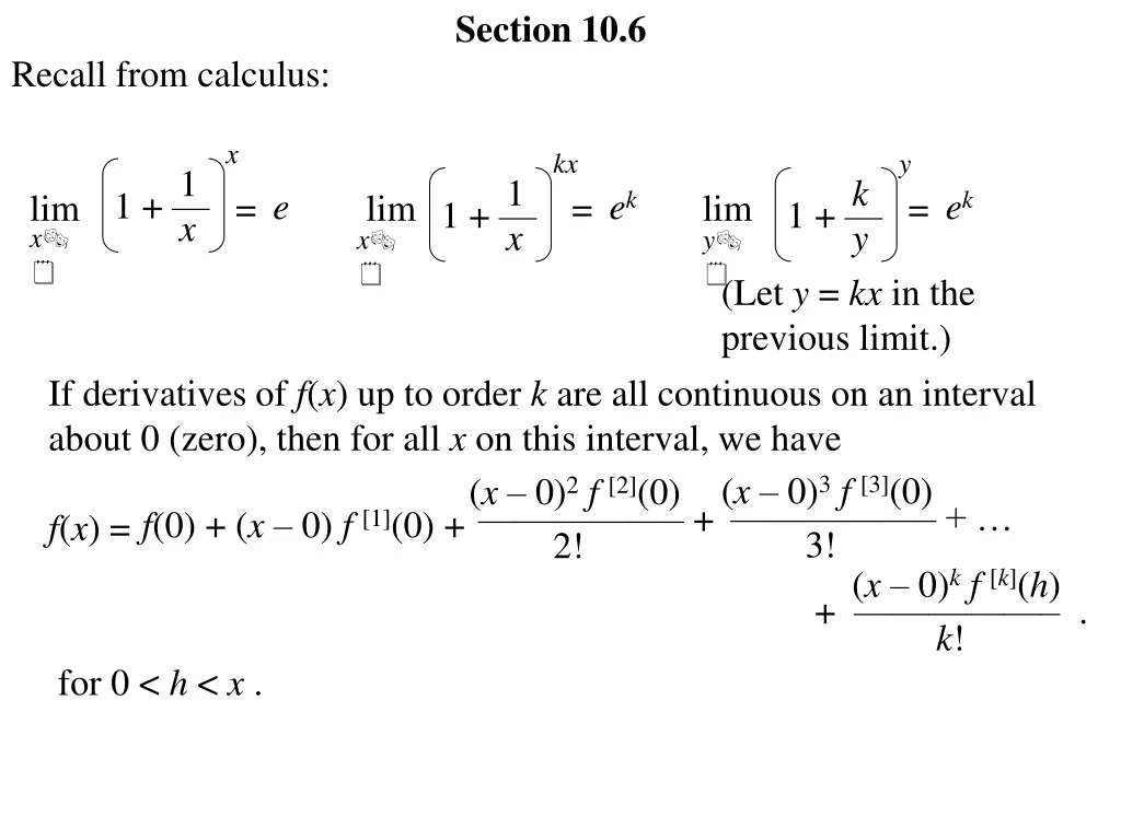
1. Section 10.6 Recall from calculus: lim = lim = lim = x kx y 1 1 + — x e ek ek 1 1 + — x k 1 + — y x x y (Let y = kx in the previous limit.) If derivatives of f(x) up to order k are all continuous on an interval about 0 (zero), then for all x on this interval, we have f(x) = (x– 0)3f[3](0) —————– + … 3! (x– 0)2f[2](0) —————– + 2! f(0) + (x– 0) f[1](0) + (x– 0)kf[k](h) + —————– . k! for 0 < h < x .

2. 1. (a) Let X1 , X2 , … , Xn be a random sample from a Bernoulli distribution with success probability p. The following random variables are defined: V = X = W = n  Xi i = 1 n  Xi– np i = 1 n  Xi i = 1 n np(1 – p) Find the m.g.f. for each of V and X. From Corollary 5.4-1, we have that (1) the m.g.f. of the random variable V = is MV (t) = (2) the m.g.f. of the random variable X = is MX (t) = n  Xi i = 1 n  (1 –p + pet) = i = 1 (1 – p + pet)n . b(n,p) (We recognize that V has a distribution.) V — n t — n MV() = (1 –p + pet / n)n .

3. (b) Find the limiting distribution for V with np equal to a given constant λ as n tends to infinity, forcing p to go to 0 (zero). Since np =  is fixed, then lim MV(t) = lim (1 –p + pet)n = n npnpet lim 1 – — + —— = nn n n n n n et lim 1 – — + —— = nn (et – 1) lim 1 + ———— = n (et – 1) e n n The limiting distribution of V is a distribution. Poisson() Consequently, for small (or large!) values of p, a binomial distribution can be approximated by a Poisson distribution with mean  = np. This should not be surprising, since the Poisson distribution was derived as the limit of a sequence of binomial distributions where p tended to zero.

4. 1.-continued (c) Find the limiting distribution for V as n tends to infinity, with p a fixed constant. lim MV(t) = lim (1 –p + pet)n =  n n We cannot find a limiting distribution for V.

5. (d) Find the limiting distribution for X as n tends to infinity, with p a fixed constant. lim MX(t) = lim (1 –p + pet/n)n = n n lim (1 – p + p[1 + t/n + (t/n)2/2! + (t/n)3/3! + …])n = n lim (1 + p[t/n + (t/n)2/2! + (t/n)3/3! + …])n = n n n pt + pt2/(2!n) + pt3/(3!n2) + … ———————————— n pt — n lim 1 + = lim 1 + = n n It is intuitively obvious that all terms in the numerator except the first go to 0 as n , and (from advanced calculus) the terms going to 0 can be ignored. ept This is the moment generating function corresponding to a distribution where the value p has probability 1 (one).

6. Suppose X1 , X2 , … , Xn is a random sample from any distribution with finite mean  and finite variance 2. Let M(t) be the common moment generating function of Xi , that is, for each i = 1, 2, …, n, we have M(t) = From Corollary 5.4-1(b), we have that the moment generating function of the random variable X = is MX(t) = tXi E(e ) n  Xi i = 1 n n  M() = i = 1 n t — n t — n M() . With M(t) and M/(t) both continuous on an interval about 0 (zero), we have that for all t on this interval, M(t) = M(0) + tM/(h) = 1 + tM/(h) for 0 < h < t .

7. Consequently, we have that for all t on this interval, MX (t) = n n t — n t — n M() = 1 + M/(h) = n t —  + n t — n 1 + [M/(h) – M/(0)] t — n for 0 < h < . To investigate the limiting distribution of X as n, we consider n [M/(h) – M/(0)] t + t ————————— n limMX (t) = lim 1 + n n It is intuitively obvious that the second term in the numerator goes to 0 as n , and (from advanced calculus) this term can be ignored. n t — = n = lim et 1 + n This is the moment generating function corresponding to a distribution where the value  has probability 1 (one).

8. Xi–  ———  For i = 1, 2, …, n, suppose Yi = , and let W = . Let m(t) be the common m.g.f. for each Yi . Then for each i = 1, 2, …, n, we have E(Yi) = m/(0) = , and Var(Yi) = E(Yi2) = m//(0) = . n  Yi i = 1 n  Xi– n i = 1 X–  = = n (n)  / n 0 1 From Theorem 5.4-1, we have that the moment generating function of the random variable W is MW(t) = n  m() = i = 1 n t — n t — n m() . With m(t) and m/(t) both continuous on an interval about 0 (zero), we have that for all t on this interval, m(t) = 1 — 2 1 — 2 m(0) + tm/(0) + t2 m//(h) = 1 + t2 m//(h) for 0 < h < t .

9. Consequently, we have that for all t on this interval, MW (t) = n n t2 — 2n t — n m() = 1 + m//(h) = n t2 — (1) + 2n t2 — 2n 1 + [m//(h) – m//(0)] t — n for 0 < h < . To investigate the limiting distribution of W as n, we consider n [m//(h) – m//(0)] t2 / 2 + (t2 / 2) ————————————– n limMW (t) = lim 1 + n n It is intuitively obvious that the second term in the numerator goes to 0 as n , and (from advanced calculus) this term can be ignored. n t2 / 2 —— = n = lim e 1 + t2 / 2 n This is the moment generating function corresponding to a standard normal (N(0,1)) distribution.

10. This proves the following important Theorem in the text: Central Limit Theorem Theorem 5.6-1

11. 1.-continued (e) Find the limiting distribution for W as n tends to infinity, with p a fixed constant. p For each i,  = E(Xi) = , and 2 = Var(Xi) = . p(1 p) From the Central Limit Theorem, we have that limiting distribution for W = is n  Xi– n i = 1 n  Xi– np i = 1 X– p —————– p(1 – p) / n = = n np(1 – p) a N(0,1) (standard normal) distribution.

12. 2. (a) (b) Suppose Y has a b(400, p) distribution, and we want to approximate P(Y 3). If p = 0.001, explain why a Poisson distribution can be expected to give a good approximation of P(Y ≥ 3), and use the Poisson approximation to find this probability. In Class Exercise #1(b), we found that the limiting distribution of a sequence of b(n, p) distributions as n tends to infinity is Poisson when np remains fixed, which forces p to tend to 0 (zero). This suggests that the Poisson approximation to a binomial distribution is better when p is close to zero (or one).  = np = (400)(0.001) = 0.4 P(Y  3) = 1 – 0.992 = 0.008 What other distribution may potentially be used to approximate a binomial probability when p is not sufficiently close to zero (or one)? The Central Limit Theorem tells us that with a sufficiently large sample size n, the normal distribution can be used.