Download
1 / 37
380 likes | 782 Views
Explore the key steps and notations in analyzing algorithm efficiency with a focus on non-recursive and recursive algorithms. Learn how to measure input sizes and running time, and analyze the time complexity of algorithms with examples. Understand worst-case, best-case, and average-case efficiency in algorithm analysis.

E N D
Fundamentals of the Analysis of Algorithm Efficiency Algorithm analysis framework Asymptotic notations Analysis of non-recursive algorithms Analysis of recursive algorithms
Expected Outcomes • The students should be able to • List the key steps in an algorithm’s analysis framework • Define the three asymptotic notations and explain their relations • Compare the asymptotic growth rate of two given functions by using the definition of asymptotic notation or Limits • Describe the key steps in analysis of a non-recursive algorithm and a recursive algorithm • Use different ways to transform a recurrence relation into its closed form • Analyze the time complexity of recursive algorithm for computing the nth Fibonacci number
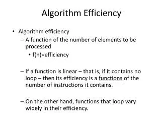
Analysis of Algorithms • Analysis of algorithms means to investigate an algorithm’s efficiency with respect tow resources: running time and memory space. Time efficiency: how fast an algorithm runs. Space efficiency: the space an algorithm requires. • Typically, algorithms run longer as the size of its input increases • We are interested in how efficiency scales wrt input size
Analysis Framework • Measuring an input’s size • Measuring running time • Orders of growth (of the algorithm’s efficiency function) • Worst-case, best-case and average-case efficiency
Measuring Input Sizes • Efficiency is defined as a function of input size. • Input size depends on the problem. • Example 1, what is the input size of the problem of sorting n numbers? • Example 2, what is the input size of adding two n by n matrices?
Units for Measuring Running Time • Should we measure the running time using standard unit of time measurements, such as seconds, minutes? • Depends on the speed of the computer. • Count the number of times each of an algorithm’s operations is executed. • Difficult and unnecessary • Count the number of times an algorithm’s basic operation is executed. • Basic operation: the operation that contributes the most to the total running time. • For example, the basic operation is usually the most time-consuming operation in the algorithm’s innermost loop.
Order of growth • Most important: Order of growth within a constant multiple as n→∞ • Example: • How much faster will algorithm run on computer that is twice as fast? • How much longer does it take to solve problem of double input size?
input size running time Number of times the basic operation is executed execution time for the basic operation Theoretical Analysis of Time Efficiency • Time efficiency is analyzed by determining the number of repetitions of the basic operation as a function of input size. Assuming C(n) = (1/2)n(n-1), how much longer will the algorithm run if we double the input size? The efficiency analysis framework ignores the multiplicative constants of C(n) and focuses on the orders of growth of the C(n). T(n) ≈ copC (n)
Worst-Case, Best-Case, and Average-Case Efficiency • Algorithm efficiency depends on the input size n • For some algorithms efficiency depends on type of input. • Example: Sequential Search • Problem: Given a list of n elements and a search key K, find an element equal to K, if any. • Algorithm: Scan the list and compare its successive elements with K until either a matching element is found (successful search) or the list is exhausted (unsuccessful search) Given a sequential search problem of an input size of n, what kind of input would make the running time the longest? How many key comparisons?
Sequential Search • Problem: Given a list of n elements and a search key K, find an element equal to K, if any. • Algorithm: Scan the list and compare its successive elements with K until either a matching element is found (successful search) or the list is exhausted (unsuccessful search)
Sequential Search Algorithm • ALGORITHM SequentialSearch(A[0..n-1], K) //Searches for a given value in a given array by sequential search //Input: An array A[0..n-1] and a search key K //Output: Returns the index of the first element of A that matches K or –1 if there are no matching elements i 0 while i < n and A[i] K do i i + 1 if i < n //A[I] = K return i else return -1
Worst-Case, Best-Case, and Average-Case • Worst case : slowest time to complete, with bad inputs chosen.For example, the worst case for a sorting algorithm might be data that's sorted in reverse order (but it depends on the particular algorithm). • Best case : fastest time to complete, with optimal inputs chosen.For example, the best case for a sorting algorithm would be data that's already sorted. • Average case : arithmetic mean. Run the algorithm many times, using many different inputs, compute the total running time (by adding the individual times), and divide by the number of trials. You may also need to normalize the results based on the size of the input sets.
Worst-Case, Best-Case, and Average-Case Efficiency • Worst case Efficiency • Efficiency (# of times the basic operation will be executed) for the worst case input of size n. • The algorithm runs the longest among all possible inputs of size n. • Best case • Efficiency (# of times the basic operation will be executed) for the best case input of size n. • The algorithm runs the fastest among all possible inputs of size n. • Average case: • Efficiency(#of times the basic operation will be executed) for atypical/randominput of size n. • NOT the average of worst and best case • How to find the average case efficiency?
Summary of the Analysis Framework • Both time and space efficiencies are measured as functions of input size. • Time efficiency is measured by counting the number of basic operations executed in the algorithm. The space efficiency is measured by the number of extra memory units consumed. • The framework’s primary interest lies in the order of growth of the algorithm’s running time (space) as its input size goes infinity. • The efficiencies of some algorithms may differ significantly for inputs of the same size. For these algorithms, we need to distinguish between the worst-case, best-case and average case efficiencies.
Orders of Growth • Three notations used to compare orders of growth of an algorithm’s basic operation count • O(g(n)): class of functions f(n) that grow no fasterthan g(n): • Ω(g(n)): class of functions f(n) that grow at least as fastas g(n) • Θ (g(n)): class of functions f(n) that grow at same rateas g(n)
>= (g(n)), functions that grow at least as fast as g(n) = (g(n)), functions that grow at the same rate as g(n) g(n) <= O(g(n)), functions that grow no faster than g(n)
0 order of growth of T(n)< order of growth of g(n) c>0 order of growth of T(n)= order of growth of g(n) ∞ order of growth of T(n) > order of growth of g(n) Using Limits for Comparing Orders of Growth limn→∞ T(n)/g(n) = • Examples: • 10n vs. 2n2 • n(n+1)/2 vs. n2 • logb n vs. logc n
f ´(n) g ´(n) f(n) g(n) lim n→∞ lim n→∞ = L’Hôpital’s rule Iflimn→∞ f(n) = limn→∞ g(n) = ∞ and the derivatives f ´, g ´ exist,Then • Example: • log2n vs. n • 2n vs. n! Stirling’s formula: n! (2n)1/2 (n/e)n
Summary of How to Establish Orders of Growth of an Algorithm’s Basic Operation Count • Method 1: Using limits. • L’Hôpital’s rule • Method 2: Using the properties • Method 3: Using the definitions of O-, -, and-notation.
Time Efficiency of Nonrecursive Algorithms Steps in mathematical analysis of nonrecursive algorithms: • Decide on parameter n indicating input size • Identify algorithm’s basic operation • Check whether the number of times the basic operation is executed depends only on the input size n. If it also depends on the type of input, investigate worst, average, and best case efficiency separately. • Set up summation for C(n) reflecting the number of times the algorithm’s basic operation is executed. • Simplify summation using standard formulas (see Appendix A)
Example 1: Maximum element • What does this algorithm compute? • What is its basic operation? • How many times is the basic operation executed? • What is the efficiency class of this algorithm?
Example 1: Maximum element • What does this algorithm compute? • Determines the largest element of the array A • What is its basic operation? • (A[i]>maxval) • How many times is the basic operation executed? • n-1 • What is the efficiency class of this algorithm? • t(n) ϵƟ(n)
Example 4: Counting binary digits It cannot be investigated the way the previous examples are. We will analyze it in the following part.
Mathematical Analysis of Recursive Algorithms • Recursive evaluation of n! • Recursive solution to the Towers of Hanoi puzzle • Recursive solution to the number of binary digits problem
Steps in Mathematical Analysis of Recursive Algorithms • Decide on parameter n indicating input size • Identify algorithm’s basic operation • Check whether the number of times the basic operation is executed may vary on different inputs of the same size. (If it may, the worst, average, and best cases must be investigated separately.) • Set up a recurrence relation and initial condition(s) for C(n)-the number of times the basic operation will be executed for an input of size n (alternatively count recursive calls). • Solve the recurrence or estimate the order of magnitude of the solution by backward substitutions or another method (see Appendix B)
Example: Factorial n!=n*(n-1)! n!=1 Recurrence relation: T(n)=T(n-1)+1 T(1)=1 Telescoping T(n)=T(n-1)+1 T(n-1)=T(n-2)+1 T(n-2)=T(n-3)+1 … T(2)=T(1)+1 Add the equations and cross equal terms on opposite sides: • T(n)=T(1)+(n-1)=n
Variation of sequential search • Given a list of n elements and a search key K, write an algorithm that find and return the number of occurrences of a given search key in the list