Download
1 / 35
430 likes | 753 Views
Simulation of a Passively Modelocked All-Fiber Laser with Nonlinear Optical Loop Mirror. Joseph Shoer ‘06 Strait Lab. Dispersion ( k ). Self-Phase Modulation n ( I ). Left : autocorrelation of sech 2 t Propagates without changing shape Could be used for long-distance data transmission.

E N D
Simulation of a Passively Modelocked All-Fiber Laser with Nonlinear Optical Loop Mirror Joseph Shoer ‘06 Strait Lab
Dispersion (k) Self-Phase Modulation n(I) • Left: autocorrelation of sech2t • Propagates without changing shape • Could be used for long-distance data transmission Solitons Direction of propagation Intensity Distance
All Fiber Laser Light from Nd:YAG Pump Laser Polarization Controller Faraday isolator Nonlinear Optical Loop Mirror 51.3% Er/Yb 48.7% Polarization Controller 90% 10% Output
Transmission Model • Different PTC at each point • Contours indicate light transmission through NOLM (value of PTC at zero input) as a function of NOLM polarization controller settings • Bright shading indicates positive PTC slope at low input • Modelocking occurs at highest low-power slope
Transmission Model • Different PTC at each point • Contours indicate light transmission through NOLM (value of PTC at zero input) as a function of NOLM polarization controller settings • Bright shading indicates positive PTC slope at low input • Modelocking occurs at highest low-power slope
Background Background Experimental Autocorrelations
Background Experimental ‘Scope Trace
Simulation Goals Gain Fiber NOLM • Model all pulse-shaping mechanisms over many round trips of the laser cavity • NOLM • Standard fiber • Er/Yb gain fiber • Model polarization dependence of NOLM (duplicate earlier model) • Duplicate lab results???
Solving Maxwell’s Equations in optical fibers yields the nonlinear Schrödinger equation (NLSE): • The NLSE can be solved numerically • Ordinary first-order solitons maintain their shape as they propagate along a fiber • Other input pulses experience variations in shape Pulse Shaping: Fibers Distance of propagation Time delay
Pulse Shaping: Fibers |E|2 Time delay |E|2 Distance of propagation Time delay Time delay
Pulse Shaping: NOLM 10 round trips Pulse edge Pulse peak 50 round trips
Pulse Shaping: Laser Gain • Pulses gain energy as they pass through the Er/Yb-doped fiber • Gain must balance loss in steady state • Gain saturation: intensity-dependent gain? • Not expected to have an effect • Gain depletion: time-dependent gain? • Not expected to have an effect • Amplified spontaneous emission (ASE): background lasing?
The Simulator Calculate PTC Repeat n times Standard Fiber (NLSE) NOLM (apply PTC) Er/Yb Fiber (NLSE + gain) Inject seed pulse Adjust gain Output pulse after i round trips
The Simulator Calculate PTC Repeat n times Standard Fiber (NLSE) NOLM (apply PTC) Er/Yb Fiber (NLSE + gain) Inject seed pulse Adjust gain Output pulse after i round trips • Power Transfer Curve is determined by polarization controller settings • Absorbs nonlinearity of NOLM fiber • Uses transmission model (Aubryn Murray ’05) fit from laboratory data
The Simulator Calculate PTC Repeat n times Standard Fiber (NLSE) NOLM (apply PTC) Er/Yb Fiber (NLSE + gain) Inject seed pulse Adjust gain Output pulse after i round trips • In the lab, pulses are initiated by an acoustic noise burst • The model uses E(0, t) = sech(t) – a soliton – as a standard input profile • This is for convenience – with enough CPU power, we could take any input and it should evolve into the same steady state result
The Simulator Calculate PTC Repeat n times Standard Fiber (NLSE) NOLM (apply PTC) Er/Yb Fiber (NLSE + gain) Inject seed pulse Adjust gain Output pulse after i round trips • 2 m of Er/Yb-doped fiber is simulated by solving the Nonlinear Schrödinger Equation with a gain term • The program uses an adaptive algorithm to settle on a working gain parameter • Dispersion and self-phase modulation are also included here • ASE is added here as a constant offset or as random noise
The Simulator Calculate PTC Repeat n times Standard Fiber (NLSE) NOLM (apply PTC) Er/Yb Fiber (NLSE + gain) Inject seed pulse Adjust gain Output pulse after i round trips • NOLM is simulated by applying the PTC, which tells us what fraction of light is transmitted for a given input intensity • This method neglects dispersion in the NOLM fiber • Fortunately, we use dispersion-shifted fiber in the loop!
The Simulator Calculate PTC Repeat n times Standard Fiber (NLSE) NOLM (apply PTC) Er/Yb Fiber (NLSE + gain) Inject seed pulse Adjust gain Output pulse after i round trips • 13 m of standard communications fiber is simulated by solving the Nonlinear Schrödinger Equation • Soliton shaping mechanisms, dispersion and SPM, come into play here • Steady-state pulse width is the result of NOLM pulse narrowing competing with soliton shaping in fibers • All standard fiber in the cavity is lumped together in the simulator
The Simulator Calculate PTC Repeat n times Standard Fiber (NLSE) NOLM (apply PTC) Er/Yb Fiber (NLSE + gain) Inject seed pulse Adjust gain Output pulse after i round trips • Output pulses from each round trip are stored in an array • We can simulate autocorrelations of these pulses individually, or averaged over many round trips to mimic laboratory measurements • Unlike in the experimental system, we get to look at both pulse intensity profiles and autocorrelation traces
The Simulator Calculate PTC Repeat n times Standard Fiber (NLSE) NOLM (apply PTC) Er/Yb Fiber (NLSE + gain) Inject seed pulse Adjust gain Output pulse after i round trips
Simulation Results I (a.u.) simulator output sech(t)2 t(ps) • Simulation for 50 round trips – results averaged over last 40 round trips • Positive PTC slope at low power • No ASE
Simulation Results I (a.u.) t(ps) • Simulation for 50 round trips – results averaged over last 20 round trips • Negative PTC slope at low power • No ASE
Simulation Results I (a.u.) t(ps) • Simulation for 50 round trips – results averaged over last 40 round trips • Positive PTC slope at low power • ASE: Random intensity noise added each round trip (max 0.016)
Simulation Results I (a.u.) t(ps) • Simulation for 50 round trips – results averaged over last 40 round trips • Positive PTC slope at low power • ASE: Random intensity noise added each round trip (max 0.016)
Simulation Results I (a.u.) t(ps) • Simulation for 50 round trips – results averaged over last 40 round trips • Positive PTC slope at low power • ASE: Constant intensity background added each round trip (0.016)
Simulation Results I (a.u.) t(ps) • Simulation for 50 round trips – results averaged over last 40 round trips • Positive PTC slope at low power • ASE: Random intensity noise added each round trip (max 0.009)
Future Work • Obtain a new transmission map so the simulator can make more accurate predictions • Produce quantitative correlations between simulated and experimental pulses • Peak intensity, background intensity, wing size • Determine the quantitative significance of simulation parameters • Are adaptive gain and amount of ASE reasonable?
Conclusions • Investigation of each mechanism in the simulator helped us better understand the laser • The simulator can produce qualitative matches for each type of pulse the laser emits – near-soliton pulses • The overall behavior of the simulator matches the experimental system and our theoretical expectations • The simulator has allowed us to explain autocorrelation backgrounds, wings, and dips as results of amplified spontaneous emission • The simulator can now be refined and become a standard tool for investigations of our fiber laser