Download
1 / 39
390 likes | 598 Views
Session 2.1 : Theoretical results, numerical and physical simulations Introductory presentation Rogue Waves and wave focussing – speculations on theory, numerical results and observations Paul H. Taylor University of Oxford. ROGUE WAVES 2004 Workshop. Acknowledgements :.

E N D
Session 2.1 : Theoretical results, numerical and physical simulationsIntroductory presentationRogue Waves and wave focussing – speculations on theory, numerical results and observationsPaul H. Taylor University of Oxford ROGUE WAVES 2004 Workshop
Acknowledgements : My students : Erwin Vijfvinkel, Richard Gibbs, Dan Walker Prof. Chris Swan and his students : Tom Baldock, Thomas Johannessen, William Bateman
This is not a rogue (or freak) wave – it was entirely expected !!
This might be a freak wave Freak ?
NewWave - Average shape – the scaled auto-correlation function NewWave + bound harmonics NewWave + harmonics Draupner wave For linear crest amplitude 14.7m, Draupner wave is a 1 in ~200,000 wave
1- and 2- D modelling • Exact – Laplace + fully non-linear bcs • – numerical • spectral / boundary element / finite element • NLEEs • NLS (Peregrine 1983) • Dysthe 1979 • Lo and Mei 1985 • Dysthe, Trulsen, Krogstad & Socquet-Juglard 2003
Perturbative physics to various orders 1st– Linear dispersion 2nd– Bound harmonics + crest/trough , set-down and return flow (triads in v. shallow water) 3rd – 4-wave Stokes correction for regular waves, BF, NLS solitons etc. 4th – (5-wave) crescent waves What is important in the field ? all of the time 1st order RANDOM field most of the time 2nd order occasionally 3rd AND BREAKING
Frequency / wavenumber focussing Short waves ahead of long waves overtaking to give focus event (on a linear basis) spectral content how long before focus nonlinearity (steepness and wave depth) In examples – linear initial conditions on ( , ) same linear (x) components at start time for several kd In all cases, non-linear group dynamics
Shallow- no extra elevation Deeper - extra elevation for more compact group Ref. Katsardi + Swan
Crest Trough Shallow Crest Trough Deep Wave kinematics – role of the return flow (2nd order)
1-D Deepwater focussed wavegroup (kd)Gaussian spectrum (like peak of Jonswap) Extra amplitude 1:1 linear focus
1-D Gaussian group– wavenumber spectra, showing relaxation to almost initial state
Numerics – discussed here • Solves Laplace equation with fully non-linear boundary conditions • Based on pseudo-spectral G-operator of Craig and Sulem (J Comp Phys 108, 73-83, 1993) • 1-D code by Vijfvinkel 1996 • Extended to directional spread seas by Bateman*, Swan and Taylor (J Comp Phys 174, 277-305, 2001) • *Ph.D. from Dept. of Civil & Environmental Eng at Imperial College, London - supervised by C. Swan • Well validated against high quality wave basin data – for both uni-directional and spread groups
2-D dominant physics is x-contraction, y-expansion Exact non-linear Linear (2+1) NLS Lo and Mei 1987
Extra elevation ? Not in 2-D 1:1 linear focus
In directionally spread interactions – permanent energy transfers (4-wave resonance) – NLEE or Zakharov eqn 2-D is very different from 1-D
Directional spectral changes – for isolated NewWave-type focussed event Similar results in Bateman’s thesis and Dysthe et al. 2003 for random field
What about nonlinear Schrodinger equation i uT + uXX - uYY + ½ uc u2 = 0 NLS-properties 1D x-long group elevation focussing - BRIGHT SOLITON 1D y-lateral group elevation de-focussing - DARK SOLITON 2D group vs. balance determines what happens to elevation focus in longitudinal AND de-focus in lateral directions
NLS modelling – conserved quantities (2-d version) useful for 1. checking numerics 2. approx. analytics
Assume Gaussian group defined byA – amplitude of group at focusSX – bandwidth in mean wave direction (also SY)gives exact solution to linear part of NLS i uT + uXX - uYY = 0 (actually this is in Kinsman’s classic book)
Assume A, SX, SY, and T/t are slowly varying 1-D x-direction FULLY DISPERSED FOCUS A-, SX -, T- AF, SXF, TF =0 similarly 1-D y-direction 2-D (x,y)-directions
Approx. Gaussian evolution 1-D x-long : focussing and contraction AF /A- = 1 + 2 -5/2 (A- / SX - )2 + …. SXF /Sx- = 1 + 2 -3/2 (A- / SX - )2 + …. 1-D y-lateral : de-focussing and expansion AF /A- = 1 - 2 -5/2 (A- / SY - )2 + …. SYF /SY- = 1 - 2 -3/2 (A- / SY - )2 + ….
Approx. Gaussian evolution • 2-D (x,y) : assume SX- = SY- = S- • AF /A- = 1 + + …. • SXF /S- = 1 + 2 -3 (A- / S-) )2 + …. • SYF /S- = 1 2 -3 (A- / S-) )2 + …. • focussing in x-long, de-focussing in y-lat, no extra elevation • much less non-linear event than 1-D (0.6 )
Conclusions based on NLS-type modelling • Importance of (A/S) – like Benjamin-Feir index • 2-D qualitatively different to 1-D • need 2-D Benjamin-Feir index, incl.directional spreading • In 2-D little opportunity for extra elevation • but changes in shape of wave group at focus • and long-term permanent changes • 2-D is much less non-linear than 1-D
‘Ghosts’ in a random sea – a warning from the NLS-equation u(x,t) = 21/2 Exp[2 I t] (1-4(1+4 I t)/(1+4x2+16t2)) t uniform regular wave t =0 PEAK 3x regular background UNDETECTABLE BEFOREHAND (Osborne et al. 2000)
Where now ? Random simulations Laplace / Zakharov / NLEE Initial conditions – linear random ? How long – timescales ? BUT No energy input - wind No energy dissipation – breaking No vorticity – vertical shear, horiz. current eddies
BUT Energy input – wind Damping weakens BF sidebands (Segur 2004) and eventually wins decaying regular wave Negative damping ~ energy input – drives BF and 4-wave interactions ?
Vertical shear Green-Naghdi fluid sheets (Chan + Swan 2004) higher crests before breaking Horizontal current eddies NLS-type models with surface current term (Peregrine)
Draupner wave – a rogue-like aspect – bound long waves Set-up NOT SET-DOWN Largest crest 2nd largest crest
Conclusions We (I) don’t know how to make the Draupner wave Energy conserving models may not be the answer Freak waves might be ‘ghosts’