Download
1 / 48
480 likes | 628 Views
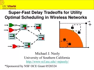
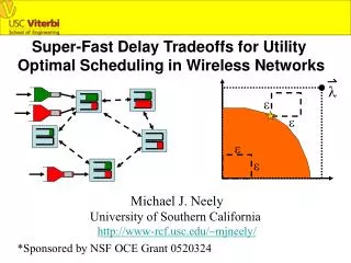
Super-Fast Delay Tradeoffs for Utility Optimal Scheduling in Wireless Networks. l. e. e. e. e. Michael J. Neely University of Southern California http://www-rcf.usc.edu/~mjneely/. *Sponsored by NSF OCE Grant 0520324. A multi-node network with N nodes and L links:. l. e. e. e.

E N D
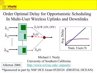
Super-Fast Delay Tradeoffs for Utility Optimal Scheduling in Wireless Networks l e e e e Michael J. Neely University of Southern California http://www-rcf.usc.edu/~mjneely/ *Sponsored by NSF OCE Grant 0520324
A multi-node network with N nodes and L links: l e e e e Slotted time t = 0, 1, 2, … t 0 1 2 3 … Traffic (An(c)(t)) and channel states S(t) i.i.d. over timeslots. Control for Optimal Utility-Delay Tradeoffs…
1) Flow Control: l e e e Ai(c) e Ri(c)(t) An(c)(t) = New Commodity c data during slot t (i.i.d) E[An(c)(t)] = ln(c) , (ln(c)) = Arrival Rate Matrix Rn(c)(t) = Flow Control Decision at (i,c): Rn(c)(t) < min[Ln(c)(t) + An(c)(t) , Rmax]
2) Resource Allocation: l e e e e Channel State Matrix:S(t) = (Sab(t)) Transmission Rate Matrix:m(t) = (mab(t)) WS(t) = Set of Feasible Rate Matrices for Channel State S. Resource allocation:choosem(t)WS(t)
mab(c)(t) < mab(t) c mab(c)(t) = 0 if (a,b) Lc 3) Routing: Lc = Set of all links acceptable for commodity c traffic to traverse Examples… mab(c)(t) = Amount of commodity c data transmitted over link (a,b)
mab(c)(t) < mab(t) c mab(c)(t) = 0 if (a,b) Lc 3) Routing: Example 1: Lc = All network links (commodity c = ) mab(c)(t) = Amount of commodity c data transmitted over link (a,b)
mab(c)(t) < mab(t) c mab(c)(t) = 0 if (a,b) Lc 3) Routing: Example 2: Lc = a directed subset (commodity c = ) mab(c)(t) = Amount of commodity c data transmitted over link (a,b)
mab(c)(t) < mab(t) c mab(c)(t) = 0 if (a,b) Lc 3) Routing: downlink uplink Example 3: Lc = Specifies a one-hop network (no routing decisions) mab(c)(t) = Amount of commodity c data transmitted over link (a,b)
mab(c)(t) < mab(t) c mab(c)(t) = 0 if (a,b) Lc 3) Routing: one-hop ad-hoc network Example 4: Lc = Specifies a one-hop network (no routing decisions) mab(c)(t) = Amount of commodity c data transmitted over link (a,b)
gn(c)(r) e e e r e Utility functions l L = Capacity region (considering all control algs.) rn(c) = Time average of Rn(c)(t) admission decisions. GOAL: (Joint flow control, resource allocation, and routing)
Network Utility Optimization: Static Optimization:(Lagrange Multipliers and convex duality) Kelly, Maulloo, Tan [J. Op. Res. 1998] Xiao, Johansson, Boyd [Allerton 2001] Julian, Chiang, O’Neill, Boyd [Infocom 2002] P. Marbach [Infocom 2002] Steven Low [TON 2003] B. Krishnamachari, Ordonez [VTC 2003] M. Chiang [Infocom 2004] Stochastic Optimization: Lee, Mazumdar, Shroff [2005] (stochastic gradient) Eryilmaz, Srikant [Infocom 2005] (fluid transformations) Stolyar [Queueing Systems 2005] (fluid limits) Neely , Modiano [2003, 2005] (Lyapunov optimization)
Network Utility Optimization: Static Optimization:(Lagrange Multipliers and convex duality) Kelly, Maulloo, Tan [J. Op. Res. 1998] Xiao, Johansson, Boyd [Allerton 2001] Julian, Chiang, O’Neill, Boyd [Infocom 2002] P. Marbach [Infocom 2002] Steven Low [TON 2003] B. Krishnamachari, Ordonez [VTC 2003] M. Chiang [Infocom 2004] Stochastic Optimization: Lee, Mazumdar, Shroff [2005] (stochastic gradient) Eryilmaz, Srikant [Infocom 2005] (fluid transformations) Stolyar [Queueing Systems 2005] (fluid limits) Neely , Modiano [2003, 2005] (Lyapunov optimization)
Our Previous Work (Neely, Modiano, Li Infocom 2005): gn(c)(r) l r Utility functions Cross-Layer Control Algorithm (with control parameter V>0): Achieves: [O(1/V), O(V)] utility-delay tradeoff!
Our Previous Work (Neely, Modiano, Li Infocom 2005): gn(c)(r) l r Utility functions Cross-Layer Control Algorithm (with control parameter V>0): Achieves: [O(1/V), O(V)] utility-delay tradeoff!
Our Previous Work (Neely, Modiano, Li Infocom 2005): gn(c)(r) l r Utility functions Cross-Layer Control Algorithm (with control parameter V>0): Achieves: [O(1/V), O(V)] utility-delay tradeoff!
Our Previous Work (Neely, Modiano, Li Infocom 2005): gn(c)(r) l r Utility functions Cross-Layer Control Algorithm (with control parameter V>0): Achieves: [O(1/V), O(V)] utility-delay tradeoff!
Our Previous Work (Neely, Modiano, Li Infocom 2005): gn(c)(r) l r Utility functions Cross-Layer Control Algorithm (with control parameter V>0): Achieves: [O(1/V), O(V)] utility-delay tradeoff!
Our Previous Work (Neely, Modiano, Li Infocom 2005): gn(c)(r) l r Utility functions Cross-Layer Control Algorithm (with control parameter V>0): Achieves: [O(1/V), O(V)] utility-delay tradeoff!
Our Previous Work (Neely, Modiano, Li Infocom 2005): gn(c)(r) any rate vector! l r Utility functions Cross-Layer Control Algorithm (with control parameter V>0): Achieves: [O(1/V), O(V)] utility-delay tradeoff!
Our Previous Work (Neely, Modiano, Li Infocom 2005): gn(c)(r) any rate vector! l r Utility functions Cross-Layer Control Algorithm (with control parameter V>0): Achieves: [O(1/V), O(V)] utility-delay tradeoff!
Our Previous Work (Neely, Modiano, Li Infocom 2005): gn(c)(r) any rate vector! l r Utility functions Achieves: [O(1/V), O(V)] utility-delay tradeoff! Uses theory of Lyapunov Optimization [Neely, Modiano 2003, 2005] Generalizes classical Lyapunov Stability results of: -Tassiulas, Ephremides [Trans. Aut. Control 1992] -Kumar, Meyn [Trans. Aut. Control 1995] -McKeown, Anantharam, Walrand [Infocom 1996] -Leonardi et. al., [Infocom 2001]
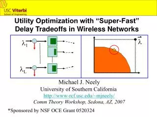
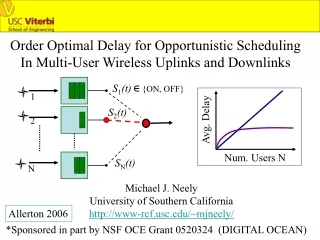
Question: Is [O(1/V), O(V)] the optimal utility-delay tradeoff? Results: For a large class of overloaded networks, we can do much better by achieving O(log(V)) average delay. l O(log(V)) Avg. Delay e e V
Question: Is [O(1/V), O(V)] the optimal utility-delay tradeoff? Results: For a large class of overloaded networks, we can do much better by achieving O(log(V)) average delay. l O(log(V)) Avg. Delay e e V
Question: Is [O(1/V), O(V)] the optimal utility-delay tradeoff? Results: For a large class of overloaded networks, we can do much better by achieving O(log(V)) average delay. l O(log(V)) Avg. Delay e e V
Question: Is [O(1/V), O(V)] the optimal utility-delay tradeoff? Results: For a large class of overloaded networks, we can do much better by achieving O(log(V)) average delay. l O(log(V)) Avg. Delay e e V
Question: Is [O(1/V), O(V)] the optimal utility-delay tradeoff? Results: For a large class of overloaded networks, we can do much better by achieving O(log(V)) average delay. l O(log(V)) Avg. Delay e e V
Question: Is [O(1/V), O(V)] the optimal utility-delay tradeoff? Results: For a large class of overloaded networks, we can do much better by achieving O(log(V)) average delay. l O(log(V)) Avg. Delay e e V
e < rn(c) < ln(c) - e Overloaded and Fully Active Assumptions: l e e e e Assumption 1 (Overloaded): Optimal operating point r* has all positive entries, and the input rate matrix l is outside of the capacity region and strictly dominates r*. That is, there exists an e>0 such that:
Overloaded and Fully Active Assumptions: l e e e e *Assumption 2 (Fully Active): All queues Un(c)(t) that can be positive are also active sources of commodity c data. *Used implicitly in proofs of conference version (Infocom 2006) but not stated explicitly. Described in more detial in JSAC 2006 (on web).
Overloaded and Fully Active Assumptions: downlink uplink l e e e e *Assumption 2 (Fully Active): All queues Un(c)(t) that can be positive are also active sources of commodity c data. *Natural assumption for overloaded one-hop networks. (Network is defined by all active links)
Overloaded and Fully Active Assumptions: one-hop ad-hoc network l e e e e *Assumption 2 (Fully Active): All queues Un(c)(t) that can be positive are also active sources of commodity c data. *Natural assumption for overloaded one-hop networks. (Network is defined by all active links)
Overloaded and Fully Active Assumptions: one-hop ad-hoc network l e e e e *Assumption 2 (Fully Active): All queues Un(c)(t) that can be positive are also active sources of commodity c data. Holds for a large class of multi-hop networks. Example: 1 or more commodities, all nodes are independent sources of each of these commodities (as in “all-to-all” traffic)
Overloaded and Fully Active Assumptions: Fully Active assumption can be restrictive in general multi-hop networks with stochastic channels: Logarithmic Utility-Delay Tradeoffs Unknown: 1 2 l1 m1(t) m2(t) Logarithmic Utility-Delay Tradeoffs Achievable: l2 1 2 l1 m1(t) m2(t)
Achieving Optimal Logarithmic Utility-Delay Tradeoffs: Automatically satisfied if we stabilize the network.
Achieving Optimal Logarithmic Utility-Delay Tradeoffs: Difficult to achieve “super-fast” logarithmic delay tradeoffs working Directly with this constraint.
Achieving Optimal Logarithmic Utility-Delay Tradeoffs: However: For any queueing system (stable or not): Un(c)(t) (actual bits transmitted)
Achieving Optimal Logarithmic Utility-Delay Tradeoffs: However: For any queueing system (stable or not): Un(c)(t) (actual bits transmitted)
Achieving Optimal Logarithmic Utility-Delay Tradeoffs: Want to Solve: We Know: Also: IF EDGE EFFECTS SMALL: Un(c)(t)
Achieving Optimal Logarithmic Utility-Delay Tradeoffs: Want to Solve: We Know: Also: IF EDGE EFFECTS SMALL: Introduce a virtual queue [Neely Infocom 2005]: Zn(c)(t)
Designing “gravity” into the system: Un(c) Q The Tradeoff Optimal Control Algorithm: Define the aggregate “bi-modal” Lyapunov Function: [Buffer partitioning Concept similar to Berry-Gallager 2002] Minimize:
Utility-Delay Optimal Algorithm (UDOA): (stated here in special case of zero transport layer storage) Flow Control (a): At node n, observe queue backlog Un(c)(t). Un(c)(t) Rn(c)(t) ln(c) Rest of Network If Un(c)(t) > Q then Rn(c)(t) = 0 (reject all new data) If Un(c)(t) < Q then Rn(c)(t) = An(c)(t) (admit all new data) (where V is a parameter that affects network delay)
Utility-Delay Optimal Algorithm (UDOA): (stated here in special case of zero transport layer storage) Flow Control (b): At node n, observe virtual queue Zn(c)(t). Un(c)(t) Rn(c)(t) ln(c) Rest of Network Then Update the Virtual Queues Zn(c)(t).
(2) Routing: Observe neighbor’s queue length Un(c)(t), compute: link (n,b) Node n cnb*(t) = Define Wnb*(t) = maxmizing weight over all c (where (n,c) Lc) Define cnb*(t) as the arg maximizer. (This is the best commodity to send over link (n,b) if Wnb*(t) >0. Else send nothing over link (n,b)).
Note: Routing Algorithm is related to the Tassiulas-Ephremides Differential backlog policy [1992], but uses weights that switch Aggressively and discontinuously ON and OFF to yield optimal delay tradeoffs. (3) Resource Allocation: Observe Channel State S(t). Choose mab(c)(t) such that
Theorem (UDOA Performance): If the overloaded And fully active assumptions are satisfied, then with Suitable choices of parameters Q, w (as functions of V), we have for any V>0: Theorem (Optimality of logarithmic delay): For one-hop networks with zero transport layer storage space (all admission/rejection decisions made upon packet arrival), then any average congestion tradeoff is necessarily logarithmic in V. (details in paper)
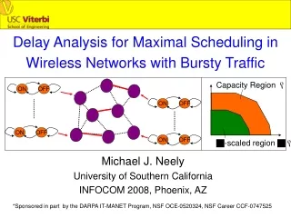
Pr[ON] = p1 l1 l2 Pr[ON] = p2 Two Queue Downlink Simulation: Observation: The coefficient Q can be reduced by a factor of 30 without Effecting edge probability, leading to further (constant factor) reductions in average delay with no affect on utility. Shown below is Reduction by 30 (original Q would have delay multiplied by 30)). input rate Simulation Utility Optimal Throughput point Bound Thruput 2 V parameter Delay (slots) “Super-Fast” Flow Control. (Input Traffic exceeds network capacity). V parameter V (Log scale x-axis) Thruput 1
Conclusions: input rate Simulation Utility Optimal Throughput point Bound V parameter Delay (slots) “Super-Fast” Flow Control. (Input Traffic exceeds network capacity). V parameter V (Log scale x-axis) Thruput 1 “Super-Fast” Logarithmic Delay Tradeoff Achievable via Dynamic Scheduling and Flow Control. 2) Logarithmic Delay is Optimal for one-hop Networks. Fundamental Utility-Delay Tradeoff: [O(1/V), O(log(V))] Novel Lyapunov Optimization Technique for Achieving Optimal Delay Tradeoffs.