Cache Models and Program Transformations
Cache Models and Program Transformations. Goal of lecture. Develop abstractions of real caches for understanding program performance Study the cache performance of matrix-vector multiplication (MVM) simple but important computational science kernel


Cache Models and Program Transformations
E N D
Presentation Transcript
Goal of lecture • Develop abstractions of real caches for understanding program performance • Study the cache performance of matrix-vector multiplication (MVM) • simple but important computational science kernel • Understand MVM program transformations for improving performance
Matrix-vector product • Code: for i = 1,N for j = 1,N y(i) = y(i) + A(i,j)*x(j) • Total number of references = 4N2 • This assumes that all elements of A,x,y are stored in memory • Smart compilers nowadays can register-allocate y(i) in the inner loop • You can get this effect manually for i = 1,N temp = y(i) for j = 1,N temp = temp + A(i,j)*x(j) y(i) = temp • To keep things simple, we will not do this but our approach applies to this optimized code as well j x i y A
Cache abstractions • Real caches are very complex • Science is all about tractable and useful abstractions (models) of complex phenomena • models are usually approximations • Can we come up with cache abstractions that are both tractable and useful? • Focus: • two-level memory model: cache + memory
Stack distance time r1 r2 Address stream from processor • r1 , r2 : two memory references • r1 occurs earlier than r2 • stackDistance(r1,r2): number of distinct cache lines referenced between r1 and r2 • Stack distance was defined by defined by Mattson et al (IBM Systems Journal paper) • arguably the most important paper in locality
Modeling approach • First approximation: • ignore conflict misses • only cold and capacity misses • Most problems have some notion of “problem size” • (eg) in MVM, the size of the matrix (N) is a natural measure of problem size • Question: how does the miss ratio change as we increase the problem size? • Even this is hard, but we can often estimate miss ratios at two extremes • large cache model: problem size is small compared to cache capacity • small cache model: problem size is large compared to cache capacity • we will define these more precisely in the next slide.
Large and small cache models • Large cache model • no capacity misses • only cold misses • Small cache model • cold misses: first reference to a line • capacity misses: possible for succeeding references to a line • let r1 and r2 be two successive references to a line • assume r2 will be a capacity miss if stackDistance(r1,r2) is some function of problem size • argument: as we increase problem size, the second reference will become a miss sooner or later • For many problems, we can compute • miss ratios for small and large cache models • problem size transition point from large cache model to small cache model
MVM study • We will study five scenarios • Scenario I • i,j loop order, line size = 1 number • Scenario II • j,i loop order, line size = 1 number • Scenario III • i,j loop order, line size = b numbers • Scenario IV • j,i loop order, line size = b numbers • Scenario V • blocked code, line size = b numbers
Scenario I • Code: for i = 1,N for j = 1,N y(i) = y(i) + A(i,j)*x(j) • Inner loop is known as DDOT in NA literature if working on doubles: • Double-precision DOT product • Cache line size • 1 number • Large cache model: • Misses: • A: N2 misses • x: N misses • y: N misses • Total = N2+2N • Miss ratio = (N2+2N)/4N2 ~ 0.25 + 0.5/N j x i y A
Scenario I (contd.) Address stream: y(1) A(1,1) x(1) y(1) y(1) A(1,2) x(2) y(1)….. y(1) A(1,N) x(N) y(1) y(2) A(2,1) x(1) y(2) • Small cache model: • A: N2 misses • x: N + N(N-1) misses (reuse distance=O(N)) • y: N misses (reuse distance=O(1)) • Total = 2N2+N • Miss ratio = (2N2+N)/4N2 ~ 0.5 + 0.25/N • Transition from large cache model to small cache model • As problem size increases, when do capacity misses begin to occur? • Subtle issue: depends on replacement policy (see next slide) j x i y A
Scenario I (contd.) Address stream: y(1) A(1,1) x(1) y(1) y(1) A(1,2) x(2) y(1)….. y(1) A(1,N) x(N) y(1) y(2) A(2,1) x(1) y(2) • Question: as problem size increases, when do capacity misses begin to occur? • Depends on replacement policy: • Optimal replacement: • do the best job you can, knowing everything about the computation • only x needs to be cache-resident • elements of A can be “streamed in” and tossed out of cache after use • So we need room for (N+2) numbers • Transition: N+2 > C N ~C • LRU replacement • by the time we get to end of a row of A, first few elements of x are “cold” but we do not want them to be replaced • Transition: (2N+2) > C N ~ C/2 • Note: • optimal replacement requires perfect knowledge about future • most real caches use LRU or something close to it • some architectures support “streaming” • in hardware • in software: hints to tell processor not to cache certain references j x i y A
Miss ratio graph 1.0 0.75 miss ratio 0.50 DDOT,b=1) 0.25 N C/2 small cache model large cache model • Jump from large cache model to small cache model will be more gradual in reality because of conflict misses
Scenario II • Code: for j = 1,N for i = 1,N y(i) = y(i) + A(i,j)*x(j) • Inner loop is known as AXPY in NA literature • Miss ratio picture exactly the same as Scenario I • roles of x and y are interchanged j x i y A
Scenario III • Code: for i = 1,N for j = 1,N y(i) = y(i) + A(i,j)*x(j) • Cache line size • b numbers • Large cache model: • Misses: • A: N2/b misses • x: N/b misses • y: N/b misses • Total = (N2+2N)/b • Miss ratio = (N2+2N)/4bN2 ~ 0.25/b + 0.5/bN j x i y A
Scenario III (contd.) Address stream: y(1) A(1,1) x(1) y(1) y(1) A(1,2) x(2) y(1)….. y(1) A(1,N) x(N) y(1) y(2) A(2,1) x(1) y(2) • Small cache model: • A: N2/b misses • x: N/b + N(N-1)/b misses (reuse distance=O(N)) • y: N/b misses (reuse distance=O(1)) • Total = (2N2+N)/b • Miss ratio = (2N2+N)/4bN2 ~ 0.5/b + 0.25/bN • Transition from large cache model to small cache model • As problem size increases, when do capacity misses begin to occur? • LRU: roughly when (2N+2b) = C • N ~ C/2 • Optimal: roughly when (N+2b) ~ C N ~ C • So miss ratio picture for Scenario III is similar to that of Scenario I but the y-axis is scaled down by b • Typical value of b = 4 (SGI Octane) j x i y A
Miss ratio graph 1.0 0.75 miss ratio 0.50 0.50 (DDOT, b=1) 0.25 0.125 (DDOT,b=4) N C/2 small cache model large cache model • Jump from large cache model to small cache model will be more gradual in reality because of conflict misses
Scenario IV • Code: for j = 1,N for i = 1,N y(i) = y(i) + A(i,j)*x(j) • Large cache model: • Same as Scenario III • Small cache model: • Misses: • A: N2 • x: N/b • y: N/b + N(N-1)/b = N2/b • Total: N2(1+1/b) + N/b • Miss ratio = 0.25(1+1/b) + 0.25/bN • Transition from large cache to small cache model • LRU: Nb + N +b = C N ~ C/(b+1) • optimal: N + 2b ~ C N ~ C • Transition happens much sooner than in Scenario III (with LRU replacement) j x i y A
Miss ratios Miss ratio 0.25(1+1/b) DAXPY 0.75/b DDOT 0.50/b 0.25/b N C/2 C/(b+1)
Scenario V • Intuition: perform blocked MVM so that data for each blocked MVM fits in cache • One estimate for B: all data for block MVM must fit in cache • B2 + 2B ~ C B ~sqrt(C) • Actually we can do better than this • Code: blocked code for bi = 1,N,B for bj = 1,N,B for i = bi,min(bi+B-1,N) for j = bj,min(bj+B-1,N) y(i)=y(i)+A(i,j)*x(j) • Choose block size B so • you have large cache model while executing block • B is as large as possible (to reduce loop overhead) • for our example, this means B~c/2 for row-major order of storage and LRU replacement • Since entire MVM computation is a sequence of block MVMs, this means miss ratio will be 0.25/b independent of N! j x i B B y
Scenario V (contd.) • Code: blocked code for bi = 1,N,B for bj = 1,N,B for i = bi,min(bi+B-1,N) for j = bj,min(bj+B-1,N) y(i)=y(i)+A(i,j)*x(j) Better code: interchange the two outermost loops and fuse bi and i loops for bj = 1,N,B for i = 1,N for j = bi,min(bi+B-1,N) y(i)=y(i)+A(I,j)*x(j) This has the same memory behavior as doubly-blocked loop but less loop overhead. j x i y A
Miss ratios Miss ratio 0.25(1+1/b) DAXPY 0.75/b DDOT 0.50/b 0.25/b Blocked N N N C/2 C/(b+1)
Key transformations • Loop permutation for i = 1,N for j = 1,N for j = 1,N for i = 1,N S S • Strip-mining for i = 1,N for bi = 1,N,B S for i = bi, min(bi+B-1,N) S • Loop tiling = strip-mine and interchange for i = 1,N for bi = 1,N,B for j = 1,N for j = 1,N S for i = bj,min(bj+B-1,N) S
Notes • Strip-mining does not change the order in which loop body instances are executed • so it is always legal • Loop permutation and tiling do change the order in which loop body instances are executed • so they are not always legal • For MVM and MMM, they are legal, so there are many variations of these kernels that can be generated by using these transformations • different versions have different memory behavior as we have seen
Matrix multiplication • We have studied MVM in detail. • In dense linear algebra, matrix-matrix multiplication is more important. • Everything we have learnt about MVM carries over to MMM fortunately, but there are more variations to consider since there are three matrices and three loops.
MMM DO I = 1, N//row-major storage DO J = 1, N DO K = 1, N C(I,J) = C(I,J) + A(I,K)*B(K,J) B K A C K IJK version of matrix multiplication • Three loops: I,J,K • You can show that all six permutations of these three loops compute the same values. • As in MVM, the cache behavior of the six versions is different
MMM DO I = 1, N//row-major storage DO J = 1, N DO K = 1, N C(I,J) = C(I,J) + A(I,K)*B(K,J) B K A C K IJK version of matrix multiplication • K loop innermost • A: good spatial locality • C: good temporal locality • I loop innermost • B: good temporal locality • J loop innermost • B,C: good spatial locality • A: good temporal locality • So we would expect IKJ/KIJ versions to perform best, followed by IJK/JIK, followed by JKI/KJI
MMM miss ratios (simulated) • L1 Cache Miss Ratio for Intel Pentium III • MMM with N = 1…1300 • 16KB 32B/Block 4-way 8-byte elements
Observations • Miss ratios depend on which loop is in innermost position • so there are three distinct miss ratio graphs • Large cache behavior can be seen very clearly and all six version perform similarly in that region • Big spikes are due to conflict misses for particular matrix sizes • notice that versions with J loop innermost have few conflict misses (why?)
IJK version DO I = 1, N//row-major storage DO J = 1, N DO K = 1, N C(I,J) = C(I,J) + A(I,K)*B(K,J) B K A C K • Large cache scenario: • Matrices are small enough to fit into cache • Only cold misses, no capacity misses • Miss ratio: • Data size = 3 N2 • Each miss brings in b floating-point numbers • Miss ratio = 3 N2 /b*4N3 = 0.75/bN (eg) 0.019 (b = 4,N=10)
IJK version (large cache) DO I = 1, N//row-major storage DO J = 1, N DO K = 1, N C(I,J) = C(I,J) + A(I,K)*B(K,J) B K A C K • Large cache scenario: • Matrices are small enough to fit into cache • Only cold misses, no capacity misses • Miss ratio: • Data size = 3 N2 • Each miss brings in b floating-point numbers • Miss ratio = 3 N2 /b*4N3 = 0.75/bN = 0.019 (b = 4,N=10)
IJK version (small cache) DO I = 1, N DO J = 1, N DO K = 1, N C(I,J) = C(I,J) + A(I,K)*B(K,J) B K A C K • Small cache scenario: • Matrices are large compared to cache • stack distance is not O(1) => miss • Cold and capacity misses • Miss ratio: • C: N2/b misses (good temporal locality) • A: N3 /b misses (good spatial locality) • B: N3 misses (poor temporal and spatial locality) • Miss ratio 0.25 (b+1)/b = 0.3125 (for b = 4)
Miss ratios for other versions DO I = 1, N//row-major storage DO J = 1, N DO K = 1, N C(I,J) = C(I,J) + A(I,K)*B(K,J) B K A C K IJK version of matrix multiplication • K loop innermost • A: good spatial locality • C: good temporal locality 0.25(b+1)/b • I loop innermost • B: good temporal locality (N2/b + N3 +N3)/4N3 0.5 • J loop innermost • B,C: good spatial locality (N3/b + N3/b + N2/b)/4N3 0.5/b • A: good temporal locality • So we would expect IKJ/KIJ versions to perform best, followed by IJK/JIK, followed by JKI/KJI
MMM experiments Can we predict this? • L1 Cache Miss Ratio for Intel Pentium III • MMM with N = 1…1300 • 16KB 32B/Block 4-way 8-byte elements
Transition out of large cache DO I = 1, N//row-major storage DO J = 1, N DO K = 1, N C(I,J) = C(I,J) + A(I,K)*B(K,J) B K A C K • Find the data element(s) that are reused with the largest stack distance • Determine the condition on N for that to be less than C • For our problem: • N2 + N + b < C (with optimal replacement) • N2 + 2N < C (with LRU replacement) • In either case, we get N ~ sqrt(C) • For our cache, we get N ~ 45 which agrees quite well with data
Blocked code As in blocked MVM, we actually need to stripmine only two loops
Notes • So far, we have considered a two-level memory hierarchy • Real machines have multiple level memory hierarchies • In principle, we need to block for all levels of the memory hierarchy • In practice, matrix multiplication with really large matrices is very rare • MMM shows up mainly in blocked matrix factorizations • therefore, it is enough to block for registers, and L1/L2 cache levels • How do we organize such a code? • We will study the code produced by ATLAS. • ATLAS also introduces us to self-optimizing programs.