Calculating  i v from the Virial EOS

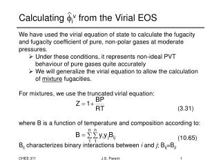
Calculating iv from the Virial EOS • We have used the virial equation of state to calculate the fugacity and fugacity coefficient of pure, non-polar gases at moderate pressures. • Under these conditions, it represents non-ideal PVT behaviour of pure gases quite accurately • We will generalize the virial equation to allow the calculation of mixture fugacities. • For mixtures, we use the truncated virial equation: • (3.31) • where B is a function of temperature and composition according to: • (10.65) • Bij characterizes binary interactions between i and j; Bij=Bji J.S. Parent

Calculating iv from the Virial EOS • Pure component coefficients (B11, B22, etc) are calculated as previously (Equations 3.48, 3.50, 3.51), and cross coefficients are found from: • (10.70) • where, • and • (10.71-75) • Bo and B1 for the binary pairs are calculated using the standard equations 3.50 and 3.51at Tr=T/Tcij. J.S. Parent

Calculating iv from the Virial EOS • We now have an equation of state that represents non-ideal PVT behaviour of mixtures: • or • We are equipped to calculate mixture fugacity coefficients from equation 10.60 J.S. Parent

Calculating iv from the Virial EOS • The result of differentiation is: • (10.69) • with the auxilliary functions defined as: • In the binary case, we have • (10.67) • (10.68) J.S. Parent

6. Calculating iv from the Virial EOS • Method for calculating mixture fugacity coefficients: • 1. For each component in the mixture, look up: • Tc, Pc, Vc, Zc,  • 2. For each component, calculate the virial coefficient, B • 3. For each pair of components, calculate: • Tcij, Pcij, Vcij, Zcij, ij • and • using Tcij, Pcij for Bo,B1 • 4. Calculate ik, ij and the fugacity coefficients from: J.S. Parent

6. Ideal Liquid Solutions • We have already developed a model for the chemical potential of ideal solutions. • Acknowledges the fact that molecules have finite volume and strong interactions, but assumes that these interactions are the same for all components of the mixture. • This are the same assumptions used in Section 7.2 for ideal mixtures of real gases. • The chemical potential of species i in an ideal solution is given by: • (10.26) • where Gil (T,P) represents the pure liquid Gibbs energy at T,P. • This reference state can be shifted to (T,unit pressure) using: • (10.37) J.S. Parent

Ideal Liquid Solutions • Substituting for Gil (T,P) yields: • To estimate the chemical potential of component i in an ideal liquid solution, all we require is the composition (xi) and the pure liquid fugacity (fil ). • The fugacity of a pure liquid can be calculated using: • (10.41) • For those cases in which the ideal solution model applies, we require only pure component data to estimate the chemical potentials and total Gibbs energy of the liquid phase. J.S. Parent

Non-Ideal Liquid Solutions • Relatively few liquid systems meet the criteria required by ideal solution theory. In most cases of practical interest, molecular interactions are not uniform between components, resulting in mixture behaviour that deviates significantly from the ideal case. • The approach for handling non-ideal liquid solutions is exactly the same as that adopted for non-ideal gas mixtures. We define a solution fugacity, fil as: • (10.42) • To use this approach, we require experimental data or correlations pertaining to the specific mixture of interest J.S. Parent

Lewis-Randall Rule • The ideal solution model developed in Sections 7.2 and 7.4 is known (in a slightly different form) as the Lewis-Randall equation: • (10.84) • The solution fugacity of component i in an ideal solution (gas or liquid) can be represented by the product of the pure component fugacity and the mole fraction. • Whenever you apply an ideal solution model, you are using the Lewis-Randall rule. • This is an approximation that yields reasonable results for similar compounds (benzene/toluene, ethanol/propanol) • However, it is important that you appreciate the limitations of this rule. When you cannot find mixture data, you may need to use it (but I suggest you look harder). J.S. Parent

Liquid Phase Activity Coefficients • Based on our definition of solution fugacity: • (10.42) • we could define a liquid phase solution fugacity coefficient: • that reflects deviations of the solution fugacity from a perfect gas mixture. • A more logical approach is to measure the deviations of the solution fugacity from ideal solution behaviour. For this purpose, we define the activity coefficient: • (10.89) • this convenient parameter is used to correlate non-ideal liquid solution data, just as i is used for gas mixtures J.S. Parent

Excess Properties of Non-Ideal Liquid Solutions • Most of the information needed to describe non-ideal liquid solutions is published in the form of the excess Gibbs energy, GE. • Excess properties are defined as the difference between the actual property value of a solution and the ideal solution value at the same T, P, and composition. • ME(T,P, xn) = M(T,P, xn) - Mid(T,P, xn) (10.86) • In defining excess properties, we use ideal solution behaviour as our reference. Pure components cannot have excess properties. • Partial excess properties can also be defined: • MiE(T,P, xn) = Mi(T,P, xn) - Miid(T,P, xn) (10.87) • where J.S. Parent

Excess Properties of Non-Ideal Liquid Solutions • The partial excess Gibbs energy is of primary interest: • where the actual partial molar Gibbs energy is provided by equation 10.42: • and the ideal solution chemical potential is: • Leaving us with the partial excess Gibbs energy: • (10.90) J.S. Parent

Excess Properties of Non-Ideal Liquid Solutions • Why do we define excess properties for liquid solutions? • They are more easily applied to experimental data • Activity coefficients can be treated as partial molar properties with respect to excess properties. Three important results follow: • (10.94) • The Gibbs-Duhem equation: • (10.98) • The summability relation, providing GE from lni data: • (10.97) J.S. Parent

Review of Thermodynamic Principles • Although thermodynamics applies to a great many problems of engineering importance, CHEE 311 focuses on phase equilibrium of multi-component systems. • In general, we are trying to describe • systems at equilibrium • How many stable phases exist, what are their compositions? • What property of the system determines its state? J.S. Parent

The Fundamental Equation • By combining the 1st and 2nd Laws, we derived the fundamental equation, which relates changes in the internal energy of a system to variations in volume, entropy and composition. • In our calculations we are most interested not in changes of V,S and composition, but P,T and composition • We therefore defined the Gibbs energy, G • The fundamental equation in terms of Gibbs energy is: • This equation is useful because it relates changes of the pressure (dP), temperature (dT) and composition (dni) of a system to changes in Gibbs energy. J.S. Parent

Chemical Equilibrium in terms of Gibbs Energy • Our first definition of chemical equilibrium is based on the total Gibbs energy (Section 4 notes, 14.1 text) • We considered a closed system (a vessel) in thermal and mechanical equilibrium with its surroundings. We charged components to the system, and watched it move towards a state of chemical equilibrium. • What is the change in Gibbs energy as it does so? • Since these changes take place spontaneously, the second law tells us that entropy must be created: • dSt + dSsurr 0 • where dSt is the entropy change of the system and dSsurr of the surroundings. • dSsurr is calculated from the heat transferred to maintain thermal and mechanical equilibrium: • dSsurr = dQsurr / T = - dQ / T J.S. Parent

Chemical Equilibrium in terms of Gibbs Energy • Substituting for dSsurr gives: • dSt -dQ / T • or • TdSt  dQ (A) • which describes the total entropy change of the system as it transfers heat to/from its surroundings in an effort to reach equilibrium. • How much heat is governed by the first law: • dQ = dUt + P dVt (B) • Substituting (A) into (B) yields, • TdSt  dUt + P dVt • or, • dUt + P dVt - TdSt  0 (14.2) J.S. Parent

Chemical Equilibrium in terms of Gibbs Energy • Equation 14.2 is a general equation which relates how the thermodynamic properties of the system change as it moves towards chemical equilibrium: • dUt + P dVt - TdSt  0 (14.2) • The Gibbs energy is defined as: • Gt = Ut + PVt - TSt • from which changes to the Gibbs energy dG are: • dGt = dUt + P dVt + VtdP - TdSt - StdT • = (dUt + P dVt - TdSt)+ VtdP - StdT • If the system approaches equilibrium at constant T,P • dGt = dUt + P dVt - TdSt • which from equation 14.2 tells us: • dGtT,P 0 (14.3) • Spontaneous changes in the composition of the system that occur at constant T,P must decrease the Gibbs energy. J.S. Parent

Equilibrium in Terms of Chemical Potential • If the approach towards equilibrium decreases the Gibbs energy, then the equilibrium state must reside at the minimum Gt. This occurs when: • dGtT,P = 0 (14.4) • If the equilibrium state is comprised of two phases (a,b), we know any change of the total Gibbs energy is: • d(nG) = d(nG)+ d(n G) • Each phase is an open system: • Therefore, changes of the total Gibbs energy at a given T,P are: • or, • or, J.S. Parent

Equilibrium in Terms of Mixture Fugacity • We have developed equations to represent the chemical potential of vapour and liquid phases. • For vapour mixtures: • For liquid mixtures: • Chemical equilibrium requires the equivalence of chemical potential for all species in both phases. Therefore, • or, • or, • Our working definition for equilibrium is now based on fugacity. J.S. Parent

Raoult’s Law • We can apply our new definition of chemical equilibrium to derive Raoult’s Law. In developing this simplified model, we assumed: • The vapour behaves as a perfect gas mixture • The liquid behaves as an ideal solution • The mixture fugacity for a perfect gas mixture is: • because iv= 1 for this simplified case. • The solution fugacity for an ideal liquid solution is: • given that i=1, isat= 1, and we ignore the pressure dependence of the Gibbs energy (Poynting factor = 1) J.S. Parent

Raoult’s Law • Given our definition of chemical equilibrium in terms of fugacity: • we can apply our simplified expressions to derive Raoult’s Law: • or • for systems where a perfect gas mixture is in equilibrium with an ideal liquid solution. • When this is not the case, we must use the full expression: J.S. Parent

Thermodynamic Calculations - Raoult’s Law • Bubble Point Pressure: • Given a liquid composition at a specified temperature, find the composition of the vapour in equilibrium and the pressure • Given T, x1, x2, ... xn find P, y1, y2,... yn • Bubble Point Temperature: • Given a vapour composition at a specified pressure, find the composition of the liquid in equilibrium and the temperature • Given P, x1, x2, ... xn find T, y1, y2,... yn • Governing Equation - Bubble Line Equation: • to find P or T • then • to find yi,…yn J.S. Parent

Thermodynamic Calculations - Raoult’s Law • Dew Point Pressure: • Given a vapour composition at a specified temperature, find the composition of the liquid in equilibrium and the pressure • Given T, y1, y2,... yn find P, x1, x2, ... xn, • Dew Point Temperature: • Given a vapour composition at a specified pressure, find the composition of the liquid in equilibrium and the temperature • Given P, y1, y2,... yn find T, x1, x2, ... xn • Governing Equation - Dew Line Equation: • to find P or T • then • to find xi,…xn J.S. Parent

Thermodynamic Calculations • “Classic” P-T Flash Calculation: • Given an overall composition at a specified temperature and pressure, find the composition of the liquid and vapour phases as equilibrium and the relative amounts of vapour and liquid • Given T,P, z1, z2,... zn find x1... xn , y1,... yn, V, L • Governing Equation - Flash equation: • to find V0 • where Ki = Pisat/P, V=vapour phase fraction • Then • to find xi,…xn • and • to find yi,…yn J.S. Parent

Calculating  i v from the Virial EOS