Object Recognition

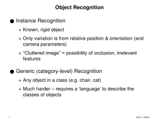
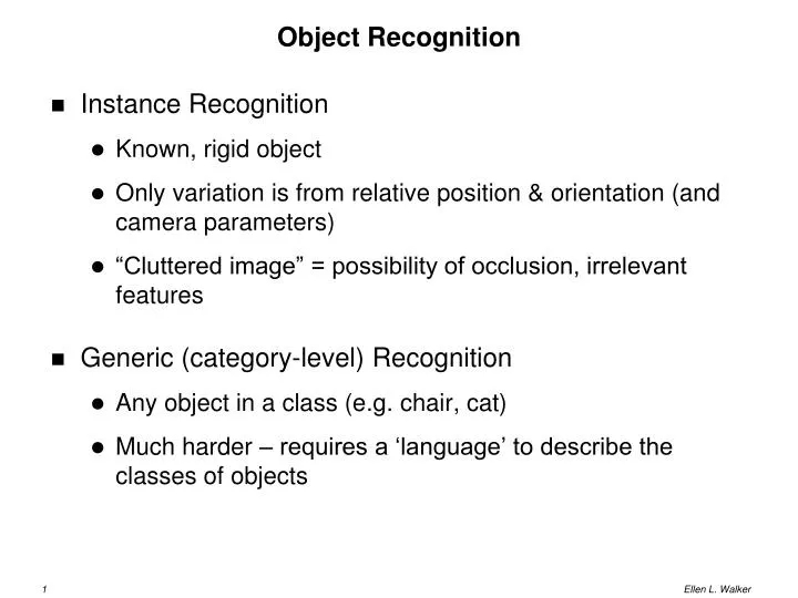
1. Object Recognition • Instance Recognition • Known, rigid object • Only variation is from relative position & orientation (and camera parameters) • “Cluttered image” = possibility of occlusion, irrelevant features • Generic (category-level) Recognition • Any object in a class (e.g. chair, cat) • Much harder – requires a ‘language’ to describe the classes of objects

2. Instance Recognition & Pose Determination • Instance recognition • Given an image, what object(s) exist in the image? • Assuming we have geometric features (e.g. sets of control points) for each • Assuming we have a method to extract images of the model features • Pose determination (sometimes simultaneous) • Given an object extracted from an image and its model, find the geometric transformation between the image and the model • This requires a mapping between extracted features and model features

3. Instance Recognition • Build database of objects of interest • Features • Reference images • Extract features (or isolate relevant portion) from scene • Determine object and its pose • Object(s) that best match features in the image • Transformation between ‘standard’ pose in database, and pose in the image • Rigid translation, rotation OR affine transform

4. What Kinds of Features? • Lines • Contours • 3D Surfaces • Viewpoint invariant 2D features (e.g. SIFT) • Features extracted by machine learning (e.g. principal component features)

5. Geometric Alignment • OFFLINE (we don’t care how slow this is!) • Extract interest points from each database image (of isolated object) • Store resulting information (features and original locations) in an indexing structure (e.g. search tree) • ONLINE (processing time matters) • Extract features from new image • Compare to database features • Verify consistency of each group of N (e.g. 3) features found from the same image

6. Hough Transform for Verificaton • Each minimal set of matches votes for a transformation • Example: SIFT features (location, scale, orientation) • Each Hough cell represents • Object center’s location (x, y) • Scale (s) • Planar (in-image) rotation (q) • Each individual feature votes for the closest 16 bins (2 in each dimension) to its own (x, y, s, q ) • Every peak in the histogram is considered for a possible match • Entire object’s set of features is transformed and checked in the image. If enough found, then it’s a match.

7. Issues of Hough-Based Alignment • Too many correspondences • Imagine 10 points from image, 5 points in model • If all are considered, we have 45 * 10 = 450 correspondences to consider! • In general N image points, M model points yields (N choose 2)*(M choose 2), or (N*(N-1)*M*(M-1))/4 correspondences to consider! • Can we limit the pairs we consider? • Accidental peaks • Just like the regular Hough transform, some peaks can be "conspiracies of coincidences" • Therefore, we must verify all "reasonably large" peaks

8. Parameters of Hough-based Alignment • How coarse (big) are the Hough space bins? • If too coarse, unrelated features will “conspire” to form a peak • If too fine, matching features will spread out and the peak will be lost • The finer the binning, the more time & space it takes • Multiple votes per feature provides a compromise • How many features needed to create a “vote”? • Minimum to determine necessary bin? • More cuts down time, might lose good information

9. More Parameters • What is the minimum # votes to align? • What is the maximum total error for success (or what is the minimum number of points, and maximum error per point)?

10. Alignment by Optimization • Need to use features to find the transformation that fits the features. • Least squares optimization (see 6.1.1 for details) • x is the feature vector from the database, • f is the transformation, • p is the set of parameters of the transformation, • x’ is the set of features from the image • Iterative and robust methods are also discussed in 6.1

11. Variations on Least Squares • Weighted Least Squares • In error equations, weight each point by reciprocal of its variance (estimate of uncertainty in the point’s location) • The less sure the location, the lower the weight • Iterative Methods (search) – see Optimization slides • RANSAC (Random Sample Consensus) • Choose k correspondences and compute a transformation. • Apply transformation to all correspondences, count inliers • Repeat many times. Result is transformation that yields the most inliers.

12. Geometric Transformations (review) • In general, a geometric transformation is any operation on points that yields points • Linear transformations can be represented by matrix multiplication of homogeneous coordinates: • Result is x’/s’ , y’/s’

13. Example transformations • Translation • Set diagonals to 1, right column to new location, all else 0 • Translation adds [dx, dy, 1]t to [x, y] • Rotation • Set upper four elements to cos(theta), -sin(theta), sin(theta), cos(theta), last element to 1, all else 0 • Scale • Set diagonals to 1 and lower right to 1 / scale factor • OR Set diagonals to scale factor, except lower right to 1 • Projective transform • Any arbitrary 3x3 matrix!

14. Combining Transformations • Rotation by  about an arbitrary point (xc, yc) • Translate so that the arbitrary point becomes 0 1 0 –xc Temp1 = 0 1 –yc x P 0 0 1 • Rotate by  cos –sin 0 Temp2 = sin cos 0 x Temp1 0 0 1 • Translate back to the original coordinates 1 0 xc Temp3 = 0 1 yc x Temp2 0 0 1

15. More generally • If T1, T2, T3 are a series of matrices representing transformations, then • T3 x T2 x T1 x P performs T1, T2, then T3 on P • Order matters! • You can precompute a single transformation matrix as T = T3 x T2 x T1 , then P' = TP is the transformed point

16. Transformations and Invariants • Invariants are properties that are preserved through transformations • Angle between two vectors is invariant to translation, scaling and rotation (or any combination thereof) • Distance between two vectors in invariant to translation and rotation (or any combination thereof) • Angle and distance preserving transformations are called rigid transformations • These are the only logical transformations that can be performed on non-deformable physical objects.

17. Geometric Invariants • Given: known shape and known transformation • Use: measure that is invariant over the transformation • The value is measurable and constant over all transformed shapes • Examples • Euclidean distance: invariant under translation & rotation • Angle between line segments: translation, rotation, scale • Cross-ratio: projective invariants (including perspective) • Note: invariants are good for locating objects, but give no transformation information for the transformations they are invariant to!

18. Cross Ratio: Invariant of Projection • Consider four rays “cut” by two lines • I = (A-C)(B-D) / (A-D)(B-C)

19. Cross Ratio Examples • Two images of one object makes 2 matching cross ratios! • Dual of cross ratio: four lines from a point instead of four points on a line • Any five non-collinear but coplanar points yield two cross-ratios (from sets of 4 lines)

20. Using Invariants for Recognition • Measure the invariant in one image (or on the object) • Find all possible instances of the invariant (e.g. all sets of 4 collinear points) in the (other) image • If any instance of the invariant matches the measured one, then you (might) have found the object • Research question: to what extent are invariants useful in noisy images?

21. Calibration Problem (Alignment to World Coordinates) • Given: • Set of control points • Known locations in "standard orientation" • Known distances in world units, e.g. mm • "Easy" to find in images • Image including all control points • Find: • Rigid transformation from "standard orientation" and world units to image orientation and pixel units • This transformation is a 3x3 matrix

22. Calibration Solution • The transformation from image to world can be represented as a rotation followed by a scale, then a translation • Pworld = TxSxRxPimage • This provides 2 equations per point • xworld = ximage*s*cos(theta) – yimage*s*sin(theta) + dx • yworld = ximage*s*sin(theta) + yimage*s*cos(theta)+ dy • Because we have 4 unknowns (s, theta, dx, dy), we can solve the equations given 2 points (4 values) • But, the relationship between sin(theta) and cos(theta) is nonlinear.

23. Getting Rotation Directly • Find the direction of the segment (P1, P2) in the image • Remember tan(theta) = (y2-y1) / (x2-x1) • Subtract the direction found from the (known) direction of the segment in "standard position" • This is theta - the rotation in the image • Fill in sin(theta) and cos(theta); now the equations are linear and the usual tools can be used to solve them.

24. Non-Rigid Transformations • Affine transformation has 6 independent parameters • Last row of matrix is fixed at 0 0 1 • We ignore an arbitrary scale factor that can be applied • Allows shear (diagonal stretching of x and/or y axis) • At least 3 control points are needed to find the transform (3 points = 6 values) • Projective transformation has 8 independent parameters • Fix lower-right corner (overall scale) at 1 • Ignore arbitrary scale factor that can be applied • Requires at least 4 control points (8 values)

25. Image Warping • Given an affine transformation (any 3x3 transformation) • Given an image with 3 control points specified (origin and two axis extrema) • Create a new image that maps the 3 control points to 3 corners of a pixel-aligned square • Technique: • The control points define an affine matrix • For each point in the new image, apply the transformation to find a point in the old image; copy its pixel value to the new image. • If the point is outside the borders of the old image, use a default pixel value, e.g. black

26. Which feature is which? (Finding correspondences) • Direct measurements can rule out some correspondences • Round hole vs. square hole • Big hole vs. small hole (relative to some other measurable distance) • Red dot vs. green dot • Invariant relationships between features can rule out others • Distance between 2 points (relative…) • Angle between segments defined by 3 points • Correspondences that cannot be ruled out must be considered (Too many correspondences?)

27. Structural Matching • Recast the problem as "consistent labeling" • A consistent labeling is an assignment of labels to parts that satisfies: • If Pi and Pj are related parts, then their labels f(Pi), f(Pj) are related in the same way • Example: if two segments are connected at a vertex in the model, then the respective matching segments in the image must also be connected at a vertex

28. Interpretation Tree (empty) A=c A=a A=b B=b B=c B=a B=c B=a B=b Each branch is a choice of feature-label match Cut off branch (and all children) if a constraint is violated

29. Constraints on Correspondences (review) • Unary constraints are direct measurements • Round hole vs. square hole • Big hole vs. small hole (relative to some other measurable distance) • Red dot vs. green dot • Binary constraints are measurements between 2 features • Distance between 2 points (relative…) • Angle between segments defined by 3 points • Higher order constraints might measure relationships among 3 or more features

30. Searching the Interpretation Tree • Depth-first search (recursive backtracking) • Straightforward, but could be time-consuming • Heuristic (e.g. best-first) search • Requires good guesses as to which branch to expand next • (Specifics are covered in Artificial Intelligence) • Parallel Relaxation • Each node gets all labels • Every constraint removes inconsistent labels • (Review neural net slides for details)

31. Dealing with Large Databases • Techniques from Information Retrieval • Study of finding items in large data sets efficiently • E.g. hashing vs. brute-force search • Example “Image Retrieval Using Visual Words” • Vocabulary Construction (offline) • Database Construction (offline) • Image Retrieval (online)

32. Vocabulary Construction • Extract affine covariant regions from image (300k) • Shape adapted regions around feature points • Compute SIFT descriptors from each region • Determine average covariance matrix for each descriptor (tracked from frame to frame) • How does this patch change over time? • Cluster regions using K-means clustering (thousands) • Each region center becomes a ‘word’ • Eliminate too-frequent ‘words’ (stop words)

33. Database Construction • Determine word distributions for each document (image) • Word frequency = (number times this word occurs) / (number words in doc) • Inverse document frequency = • Log (number of documents containing this word) / (number of documents) • tf-idf measure • (word freq) * (inverse doc freq) • Each document is represented by a vector of tf-idf measures for each word

34. Image Retrieval • Extract regions, descriptors, and visual words • Compute tf-idf vector for the query image (or region) • Retrieve candidates with most similar tf-idf vectors • Brute force, or using an ‘inverse index’ • (Optional) re-rank or verify all candidate matches (e.g. spatial consistency, validation of transformation) • (Optional) expand the result by submitting highly-ranked matches as new queries • (OK for <10k keyframes, <100k visual words)

35. Improvements • Vocabulary tree approach • Instead of ‘words’, create ‘vocabulary tree’ • Hierarchical: each branch has several prototypes • In recognition, follow the branch with the closest prototype (recursively through the tree) • Very fast: 40k CD’s recognized in real time (30/sec); 1M frames at 1Hz (1/sec) • More sophisticated data structures • K-D Trees • Other ideas from IR • Very active research field right now

36. Application: Location Recognition • Match image to location where it was taken • E.g. annotating Google Maps, organizing information on Flickr, star maps • Match via vanishing points (when architectural objects are prominent) • Find landmarks (the ones everyone photographs) • Identify automatically as part of indexing process • Issues: • large number of photos • Lots of ‘clutter’ (e.g. foliage) that doesn’t help recognition

37. Image Retrieval • Determine the tf-idf measure for the image (using words already included in the database) • Match to the tf-idf measures for images in the DB • Similarity measured by normalized dot product (more similar = higher) • Difference measured by Euclidean distance