COMPRESSIVE SENSING IN DT-MRI

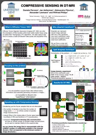
1. Results for DT MRI COMPRESSIVE SENSING IN DT-MRI Daniele Perrone1, Jan Aelterman1, Aleksandra Pižurica1, Alexander Leemans2 and Wilfried Philips1 1 Ghent University - TELIN - IPI – IBBT - St.-Pietersnieuwstraat 41, B-9000 Gent, Belgium 2 Image Sciences Institute - University Medical Center - Heidelberglaan 100, 3584 Utrecht, the Netherlands. daniele.perrone@telin.ugent.be What is Diffusion Tensor MRI? Why shearlet transform? Diffusion Tensor Magnetic Resonance Imaging (DT- MRI) can infer the orientation of fibre bundles within brain white matter tissue using so-called Fiber Tractography (FT) algorithms. The data capture step force to choose a trade off between data quality and acquisition time. Shearlets can represent natural image optimally with only a few significant (non-zero) coefficients, while noise and corruptions would need more coefficients. We can force a noise and artifact free reconstruction. f is C² (edges:piecewise C²) Approximation error: Fourier basis : εM ≤ C * M -1/2 Wavelet basis : ε M ≤ C * M -1 Shearlet tight frame : ε M ≤ C * (log(M))3 * M-2 MRI scanner Full brain acquisition ( axial view ) Brain tractography ( coronal view ) Fiber Tract. Split Bregman technique Formalization of the problem : x* = argmin |Sx| so that ||y – Fx||2 x IFFT * N ( N different directions ) xi+1 = argmin λ/2||Fx - yi||2 + μ/2||di - Sx -μi||2 di+1 = argmin |d| + μ/2||d - Sxi+1 - μi||2 μ=μi + Sxi+1 - di+1 goto 1 until convergence of μi+1 yi+1 = yi + y - Fxi+1 goto 1 until convergence of yi+1 1 x 2 d Split Bregman algorithm : 3 4 5 Focusing on the problem It is not possible to acquire fewer data without losing information and eventually generating corruption in images... …is it possible to discard only “superfluous” information? 6 CS No artifacts Image domain: experiment 50% of the coefficients used PSNR of the reconst. image: 40 dB Gibbs artifact : ABSENT Theoretical acquisition speedup: 2 The color image IFFT Gibbs ringing artifact in IMAGE DOMAIN IFFT Fiber Tractography SEED (corpus callosum - sagittal view) Wrong - even negative ! - eigenvalues in DIFFUSION TENSOR DOMAIN Brain tracts ( coronal view ) Fiber Tract. FFT Speeding up with Compressive Sensing • Considering just the Fourier samples that are not attenuated: • the number of samples is less than the number of • image pixels an infinite number of possible • image reconstructions; • naively filling in the missing data in Fourier space leads • to artifacts in MRI and therefore in FT reconstruction; • proposed: Compressive Sensing (CS) reconstruction • we have an infinite number of possible image reconstructions • we do want to maintain fidelity to the acquired data • we can choose the image that is representable with the LOWEST number of coefficients possible in the shearlet domain ( that corresponds to the minimum number of • image structures ) Fiber Tract. 50% FFT Compr. Sensing K-space reconstruction Fiber Tract. Promising quantitative improvements considering : - number of fiber tracts - mean length of the fiber tracts - fractional anisotropy - apparent diffusion coefficient - mean value and variance of the three eigenvalues