Download
1 / 38
410 likes | 700 Views
Object Recognition. Outline: Introduction Representation: Concept Representation: Features Learning & Recognition Segmentation & Recognition. Credits: major sources of material, including figures and slides were:

E N D
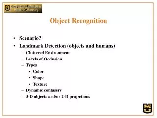
Object Recognition • Outline: • Introduction • Representation: Concept • Representation: Features • Learning & Recognition • Segmentation & Recognition
Credits: major sources of material, including figures and slides were: • Riesenhuber & Poggio, Hierarchical models of object recognition in cortex. Nature Neuroscience, 1991. • B. Mel. SeeMore. Neural Computation, 1997. • Ullman, Vidal-Naquet, Sari. Visual features of intermediate complexity and their use in classification. Nature Neuroscience, 2002. • David G. Lowe. Distinctive Image Features from Scale-Invariant Keypoints. Int. J. of Computer Vision, 2004. • and various resources on the WWW
position/pose/scale lighting/shadows articulation/expression partial occlusion Why is it difficult? Because appearance drastically varies with: need invariant recognition!
The “Classical View” Historically: Feature Extraction Segmentation Recognition Image Problem: Bottom-up segmentation only works in very limited range of situations! This architecture is fundamentally flawed! Two ways out: 1) “direct” recognition, 2) integration of seg.&rec.
Ventral Stream V1 V2 V4 IT edges, bars objects, faces → larger RFs, higher “complexity”, higher invariance → K.Tanaka (IT) D.vanEssen (V2)
Basic Models seminal work by Fukushima, newer version by Riesenhuber and Poggio
Questions • what are the intermediate features? • how/why are they being learned? • how is invariance computation implemented? • what nonlinearities; at what level (dendrites?) • how is invariance learned? • temporal continuity; role of eye movements • basic model is feedforward, what do feedback connections do? • attention/segmentation/bayesian inference?
Representation: Concept • 3-d models: won’t talk about • view-based: • holistic descriptions of a view • invariant features/histogram techniques • spatial constellation of localized features
Holistic Descriptions I:Templates Idea: • compare image (regions) directly to template • image patches, object template are represented as high-dimensional vectors • simple comparison metrics (Euclidean distance, normalized correlation, ...) Problem: • such metrics not robust w.r.t. even small changes in position/aspect/scale changes or deformations • difficult to achieve invariance
Holistic Descriptions II:Eigenspace Approach Somewhat better:“Eigenspace” approaches • perform Principal Component Analysis (PCA) on training images (e.g. “Eigenfaces” • compare images by projecting on subset of the PCs Murase&Nayar (1995) Turk&Pentland (1992)
Assessment • quite successful for segmented and carefully aligned images (e.g., eyes and nose are at the same pixel coordinates in all images) • but similar problems as above: • not well-suited for clutter • problems with occlusions • some notable extensions trying to deal with this (e.g., Leonardis, 1996,1997)
Feature Histograms Idea: reach invariance by computing invariant features Examples: Mel (1997), Schiele&Crowley (1997,2000) histogram pooling: throw occurrences of simple feature from all image regions together into one “bin”
Assessment: • works very well for segmented images with • only one object, but... Problem: • histograms of simple features over the whole image leads to a“superposition catastrophe”, lacks a “binding” mechanism • consider several objects in scene: histogram contains all their features; no representation of which features came from same object • system breaks down for clutter or complex backgrounds
Training and test images, performance: A B C D E
Elastic Matching Techniques: • Fischler&Elschlager (1973), Lades et.al. (1993) • Tremendously successful for: • face finding/recognition • object recognition • gesture recognition • cluttered scene analysis “Elastic Graph Matching” (EGM) Feature Constellations Observation: holistic templates and histogram techniques can´t handle cluttered scenes well Idea: How about constellations of features? E.g. face is constellation of eyes, nose, mouth, etc.
Representation: Features Only discuss local features: • image patches • wavelet basis, e.g., Haar, Gabor • complex features, e.g., SIFT (= Scale Invariant Feature Transform)
Image Patches Ullman, Vidal-Naquet, Sali (2002) “merit”: likelihood ratio: weight:
Gabor Wavelets image space frequency space • in frequency space Gabor wavelet is a Gaussian • “wavelet”: different wavelets are scaled/rotated versions of a mother wavelet
Gabor Wavelets as filters Gabor filters: sin() and cos() part compute correlation of image with filter at every location x0:
Tiling of frequency space: Jets measured frequency tuning of biological neurons (left) and dense coverage applying different Gabor filters (with different k) to same image location gives vector of filter responses: Jet
SIFT Features • step 1: find scale space extrema
step 3: local image descriptor extracted at key points is a 128-dim vector
Learning and Recognition • top-down model matching • Elastic graph matching • bottom-up indexing • with or without shared features
Elastic Graph Matching (EGM) “view based”: need different graphs for different views Representation: graph nodes labelled with Jets (Gabor filter responses of different scales/orientations) Matching: Minimize cost function that punishes dissimilarities of Gabor responses and distortions of the graph through stochastic optimization techniques
Bunch Graphs Idea: add invariance by labelling graph nodes with collection or bunch of different feature exemplars (Wiskott et.al.,1995, 1997) Advantage: can decouple finding the facial features from the identification Matching uses a MAX rule.
Indexing Methods • when you want to recognize very many objects, it’s inefficient to individually check for each model by searching for all of its features in a top-down fashion • better: indexing methods • also: share features among object models
Recognition with SIFT features • recognition: extract SIFT features; match to nearest neighbor in data base of stored features; use Hough transform to pool votes
Scaling Behavior when Sharing Features between models • Recognition speed limited more by number of features rather than number of object models, modest number of features o.k. • can incorporate many feature types • can incorporate stereo (reasoning about occlusions)
Hierarchies of Features • Long history of using hierarchies: • Fukushima’s Neocognitron (1983), • Nelson&Selinger (1998,1999): • Advantages using hierarchy: • faster learning and processing • better grip on correlated • deformations • easier to find proper specificity • vs. invariance tradeoff?
Feature Learning • Unsupervised clustering: not necessarily optimal for discrimination • Use big bag of features, fish out the useful ones (e.g. via boosting: Viola, 1997): takes very long to train, since you have to consider every feature from that big bag • Note: usefulness of one feature depends on the which other ones you’re using already. • Learn higher level features as (nonlinear) combinations of lower level features (Perona et.al., 2000): also takes very long to train, only up to 5 features. But could use locality constraint
Feedback Question: Why all the feedback connections in the brain? Important for on-line processing? Neuroscience: Object recognition in 150 ms (Thorpe et.al., 1996), but interesting temporal response properties of IT neurons (Oram&Richmond, 1999); some V1 neurons “restore” line behind an occluder Idea: Feed-forward architecture: can’t correct errors made at early stages later on. Feedback architecture can! “High level hypotheses try to reinforce their lower level evidence while hypotheses compete at all levels.”
Recognition & Segmentation • Basic Idea: integrate recognition with segmentation in a feedback architecture: • object hypotheses reinforce their supporting evidence and inhibit competing evidence, suppressing features that do not belong to them (idea goes back to at least the PDP books) • at the same time: restore missing features due to partial occlusion (associative memory property)
Current work in this area • mostly demonstrating how recognition can aid segmentation • what is missing is a clear and elegant demonstration of a truly integrated system that shows how the two kinds of processing help each other • Maybe don’t treat as two kinds of processing but one inference problem • how best to do this? “million dollar question”