Download
1 / 52
520 likes | 542 Views
This chapter explores the vorticity equation for a layer of homogeneous fluid with variable depth and its applications, with a focus on planetary waves in the atmosphere. The chapter discusses the beta-plane approximation, non-divergent motions, mathematical analysis of the waves, and the dynamics of a basic westerly airflow.

E N D
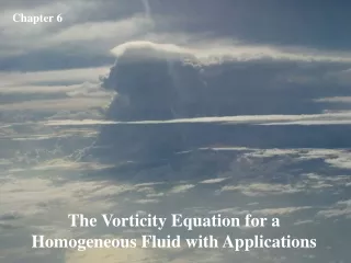
Chapter 6 The Vorticity Equation for a Homogeneous Fluid with Applications
The vorticity equation for a layer of homogeneous fluid of variable depth H(x,y) H(x,y) X body force per unit mass horizontal momentum equations
Cross-differentiation Continuity equation Integrate with respect to height Assume u and v to be functions of x and y only
Use the identity In the special case whereX = 0, The quantity (f + z)/H is called the potential vorticity for a homogeneous fluid. It is conserved following a fluid column.
Planetary, or Rossby Waves • The atmosphere is a complex dynamical system which can support many different kinds of wave motion covering a wide range of time and space scales. • One of the most important wave types as far as the large-scale circulation of the atmosphere is concerned is the planetary wave, or Rossby wave. • These are prominent in hemispheric synoptic charts; either isobaric charts at mean sea level (msl) or upper level charts of the geopotential height of isobaric surfaces, e.g., 500 mb.
Southern hemisphere mean sea level isobaric analysis on a stereographic projection illustrating the wavy nature of the flow in the zonal direction.
The 500 mb analysis corresponding to the previous one. Isopleths of the 500 mb surface are given in decametres.
Regional 500 mb analysis showing planetary-scale waves. Broken lines are isotachs in knots (2 kn = 1 ms-1). Note the two “jet-streaks”, one just southwest of Western Australia, the other slightly east of Tasmania.
Planetary Waves are Inertial Waves • A planetary wave in its pure form is a type of inertial wave which owes its existence to the variation of the Coriolis parameter with latitude. • An inertial wave is one in which energy transfer is between the kinetic energyof relative motion and kinetic energy of absolute motion. • Such waves may be studied within the framework of the Cartesian equations described above by making the so-called "beta-plane" or "b-plane" approximation.
The beta-plane approximation • This approximation regards f as a linear function of the north-south direction y, i.e., f = f0 + by, where b is a positive constant, so that the effect of the variation of the Coriolis parameter with latitude is incorporated in the vorticity equation. • The beta-plane approximation allows us to study of the effects of varying f with latitude without the added complication of working in spherical geometry.
Non-divergent motions • A simple description of the basic dynamics of a pure horizontally nondivergent planetary wave may be given by considering two-dimensional flow on a beta plane: • i.e., in a rectangular coordinate system with x pointing eastwards, y pointing northwards, and with f = f0 + by. • Horizontal nondivergence implies that H is a constant and therefore, in the absence of a body force, the vorticity equation reduces to The absolute vorticity of each fluid column remains constant throughout the motion.
Non-divergent Rossby waves y (north) B Each particle displacement conserves f + z D C cp A x (east) Diagram illustrating the dynamics of a nondivergent Rossby wave Northern hemisphere
Mathematical analysis • Two-dimensionality implies that there exists a streamfunctionysuch that a PDE withyas the sole dependent variable. For small amplitude motions, the equation can be linearized For motions independent of y (thenu = -yy º 0), there exist travelling wave solutions of the form
wherek, wand are constants. • kis called thewavenumberandwthefrequency • The wavelengthisl = 2p/kand theperiodT = 2p/w • Thephase speedof the wave in thex-directionis cp= w/k. Substitution ofyinto for a nontrivial solution : This is thedispersion relationfor the waves.
Thephase speedof the wave in thex-directionis: • Sincecpis a function ofk(orl),the waves are calleddispersive. • In this case, the longer waves travel faster than the shorter waves. • Notice thatb > 0implies thatcp < 0and hence the waves traveltowards the west, consistent with physical arguments. The perturbation northward velocity component is This is exactly 90 deg. out of phase with y.
The mean kinetic energy density averaged over one wavelength (or period) is: For a given wave amplitude the shorter waves (largerk) are more energetic.
A basic westerly airflow • Suppose now there is a basic westerly airflow(U, 0), Ubeing a constant. • Remember westerly means from the west; it is sometimes called a zonal flow. • Thenu × slinearizes to U¶/¶xand Travelling wave solutions of the type exist as before: The dispersion relation is: w = Uk -b/k
Thus the waves are simply advected with the basic zonal flow. • The above equation is known as Rossby's formula. • It shows that waves propagate westwards relative to the air at a speed proportional to the square of the wavelength. • In particular, waves are stationary when ks = (b/U) • They move westwards forl > ls = 2p/ks and eastwards forl < ls
Planetary waves around the earth • If a planetary wave extends around the earth at latitude F, its wavelength cannot exceed the length of that latitude circle, 2pa cos F , a being the earth's radius. • For n waves around the latitude circle at 45° on which b = f/a, then: with corresponding period T = 2p/|w| = 2pn/W. • SinceW = 2p/(1 day), the period is simply n days.
Values ofl, Tandcpin the caseU = 0are listed in the table for values ofnfrom1to5. • Fornequal to1or 2,cpis unrealistically large. => This results from the assumption of nondivergence, which is poor for the ultra-long waves.
The stationary wavelengthslsfor various flow speedsU, calculated from the formula are listed below forbas 1.6 x 10⁻¹¹ m -1s -1, appropriate to45deg. latitude.
Planetary waves in the atmosphere • Hemispheric upper air charts such as those at 500 mb show patterns with between about 2 and 6 waves. • These waves are considered to be essentially planetary waves forced by three principal mechanisms: • orographic forcing resulting from a basic westerly air stream impinging on mountain ranges such as the Rockies and Andes; • thermal forcing due to longitudinal heating differences associated with the distribution of oceans and continents: and • nonlinear interaction with smaller scale disturbances such as extra-tropical cyclones.
Planetary waves in the oceans • Planetary waves have been identified in the oceans also. • They are thought to be driven, inter alia, by fluctuating wind stresses at the ocean surface.
Large scale flow over a mountain barrier the lee trough plan view U side view tropopause U uniform upstream flow with z = 0 One layer model for uniform westerly flow over topography (NH- case).
For relatively narrow mountain ranges, such as the Southern Alps of New Zealand, the pattern of flow deflection is recognizable mainly in the vicinity of the mountains. • For continental scale orography, such as the Rocky mountains and Tibetan Plateau, the influence is almost certainly felt over the entire hemisphere. • Thus orography is believed to be an important factor in generating stationary planetary waves of low wavenumber.
The surface isobar pattern around New Zealand during northwesterly flow ahead of an approaching cold front. Note the strong deflection of the isobars produced by the orography. Remember f < 0 in the southern hemisphere - hence the sense of the deflection!
Owing to the relatively small horizontal scale of the mountain barrier in New Zealand, the beta effect is likely to be small compared, say, with deflections produced by the Rocky mountains. • In the latter case, the lee trough may be a significant synoptic scale feature at upper levels and therefore, according to Sutcliffe's theory (see Chapter 9), we expect there to exist a favourable region for cyclogenesis just ahead of the trough. • This is borne out by observations, and depressions which form or intensify there are called 'lee cyclones'. • Lee cyclogenesis is a common occurrence in the Gulf of Genoa region when a northwesterly airstream impinges on the European Alps.
Easterly flow over a mountain barrier • The situation concerning easterly flow across a mountain barrier is tricky because of upstream influence effects; see Holton 4.3, especially page 90 and Holton (1993). • The latter reference contains an excellent review of the dynamics of stationary planetary waves.
Wind driven ocean currents • The potential vorticity equation for a homogeneous fluid is helpful in understanding the pattern of wind driven surface currents in the ocean. • The next figure shows the major surface currents of the world oceans (After Somerville and Woodhouse, 1950; see article by Longuet-Higgins, 1965).
Summary of the main features • To some extent the currents follow the mean winds; those flowing westwards in sub- tropical latitudes follow the easterly trade winds while those flowing eastwards follow the westerly winds in middle latitudes. • Most of the strongest currents occur in the neighbourhood of western boundaries, for example: • The Gulf Stream in the North Atlantic • The Kuroshio in the North Pacific • The Somali Current (which is seasonal) in the Indian Ocean • The Brazil Current, and • The East Australian Current.
North Atlantic currents Streamlines of mean winds in the North Atlantic (broken lines), and of mean surface currents, as represented by the isotherms (full lines) (after Stommel, 1958).
Assumptions • It is observed that most of the wind-driven circulation takes place in a shallow surface layer above the main thermocline. • We shall ignore the details of • the slow internal circulation in the deep ocean • the variations in density • the variations in bathymetry (sea depth below mean sea level) • We shall consider only mean horizontal velocities, averaged vertically between the free surface down to some uniform reference depth H, below which steady transports are assumed negligible.
In the absence of any body forces and with H constant, the absolute vorticityf + z is conserved following a fluid parcel. • If a parcel moves equatorwards, the planetary vorticity decreases and hence its relative vorticity increases. • In other words, the parcel finds the earth "spinning more slowly" beneath it and so appears to spin faster (in a cyclonic sense) relative to the earth. • Suppose a wind-stress t(x,y) per unit area acts on the ocean surface. • We may regard this as equivalent to a body force t(x,y)/rH per unit mass, distributed uniformly over depth.
Then • In the ocean interior, i.e., away from the boundaries of the continents,z ~ 10-1 ms-1/1000 km = 10-7 s << f = 10-4 s-1. • Assume that internal friction is small compared with wind stresses, then for steady currents there is an approximate balance between the wind stress curl and the increase in planetary vorticity due to meridional motion.
Sverdrup flow The new vorticity injected by the wind stress is compensated by a meridional motion v to a latitude where its planetary vorticity just "fits in" with the change in f. Sinceb = df/dy • This result is due to the well-known Swedish oceanographer H.U. Sverdrup (1888-1957). • In the North Atlantic between 20°N and 50°N, b > 0 and k curl t < 0 so that the motion over nearly all the ocean will be towards the south, a result which accords with the figure.
The return flow • Mass conservation requires that there be a return flow. • This must occur near a boundary where the assumptions (principally the neglect of friction) under which Sverdrup’sequation was derived are no longer valid. • Moreover, in the return flow, the planetary vorticity tendency is positive so there must be an input of vorticity, presumably frictional at the boundary, to satisfy • Thus, we expect an intense northward current somewhere along the margin of the ocean into which cyclonic vorticity is diffused from the boundary. • The question is: which side of the ocean?
Which side of the ocean? Eastern boundary Western boundary Wrong sign! Correct sign! • Cyclonic vorticity is diffused from a western boundary. • We surmised that the principal vorticity balance in the boundary current is between the planetary vorticity tendency and the frictional rate of generation.
At what latitude does the return flow occur? • A further question is: at what latitude should the boundary current leave the coast? • To explore this question, let us suppose that the wind stress t= (t(y), 0). Then Using this together with the continuity equation gives
At an eastern boundary u = 0 and hence sgn (u) depends on sgn (¶u/¶x). • If tyy > 0, u < 0 and streamlines run into the western boundary layer • On the other hand, if tyy < 0, u > 0 and streamlines leave the western boundary layer. • Hence the critical latitude is where tyy = 0, which for the North Atlantic is at about 30°N, just about where the Gulf Stream leaves the coast. • Of course, bottom topography may also play a role in determining the critical latitude and this has not been taken into account in the foregoing simple analysis.
Other effects • In the analysis presented above, the currents are assumed to be depth independent, but observations show that this is not always a good approximation; often there are counter currents at larger depths and this is certainly true of the Gulf Stream. • Thus the theory really applies to the net mass transports. Also, transient effects may be important. • For example, the Somali Current in the Indian Ocean undergoes a pronounced annual variation due to monsoonal wind changes. • More important, transient currents may be an order of magnitude larger than steady mean currents and may have a significant overall effect on the dynamics through nonlinear processes.
Topographic waves • We have seen that the dynamics of Rossby waves can be understood in terms of the conservation of absolute vorticity f + z, as fluid parcels are displaced meridionally. • More generally, for a fluid of variable depth h, it is the potential vorticity (f + z)/h which is conserved. • Thus if the depth of the fluid column varies during the motion, changes in z are induced, even if f is a constant (i.e., if there is no b-effect), and wave motions analogous to planetary waves may occur. • These are called topographic waves, or if b ¹ 0, Rossby-topographic waves.
We consider here the case b = 0. • The potential vorticity equation may be written Dz/Dt = {(f + z)/h} Dh/Dt which gives, on linearization about a state of zero motion, where h0 is some reference depth. • This equation has the interpretation that the local rate of change of vorticity is equal to the rate of vorticity production by vortex line stretching caused by the advection of fluid across the depth contours.
A simple example is that of topography h = h0e-my with m > 0. y x h ho
We consider motions which are independent of y. Then reduces to This is identical in form with when¶ /¶y º 0, remembering that v = ¶y/ ¶x. • It follows that the dynamics is similar to that of planetary waves with f playing the role of b, and there exists a travelling wave solution of the form
Hence decreasing depth (in the ocean, for example) plays a role analogous to that of increasing Coriolis parameter. • There is one essential difference between this and the earlier problem. Here, continuity => whereupon
This cross motion is necessary to offset the divergence which occurs as fluid columns move across the depth contours. • Recall that, at middle latitudes, b ~ f/a. Thus the effect of bottom topography and b will be comparable, leading to a so-called mixed Rossby-topographic wave, if fm ~ b, i.e., if m ~ 1/a. • There are many areas in the ocean where bathymetric slopes far exceed the critical slope given by fh-1dh/dy ~ b, and in such regions, the beta effect is completely swamped by that of bottom topography, assuming of course that the motions are barotropic; that is they are uniform all the way to the ocean floor.
Continental shelf waves • A particular example of topographic waves is that of shelf waves. • These are a type of "edge wave" which owe their existence to the sloping continental shelf linking the coast with the deep ocean floor, sometimes referred to as the abyssal plain. • See next figure =>
Continental shelf waves column motions are mainly normal to the coast, but the wave propagates along the coast land sea typically 4 km shelf abyssal plain typically 100 km Flow configuration for a model for continental shelf waves.
Continental shelf waves are observed off the east coast of Australia, for example. They have a period (2p/w) of a few days. • At Sydney, shelf waves propagate with a speed of about 2.8 ms-1 (240 km/day). • They are believed to be generated by the passage of synoptic scale meteorological disturbances across the coast.