Distributed Algorithms for Guiding Navigation across a Sensor Network
This paper presents distributed algorithms designed to guide mobile devices through sensor networks, ensuring a safe distance from danger areas. It introduces three main algorithms: motion planning using artificial potential fields, dynamic programming for determining the safest path, and a navigation algorithm for path retrieval. The study analyzes the algorithms' performance, examines various adaptation measures, and provides experimental results based on a network of Mote sensors. Findings highlight the algorithms' efficiency in propagating information, adapting to network changes, and finding optimal paths in real-time scenarios.

Distributed Algorithms for Guiding Navigation across a Sensor Network
E N D
Presentation Transcript
Distributed Algorithms for Guiding Navigation across aSensor Network Qun Li, Michael De Rosa, and Daniela Rus Department of Computer Science Dartmouth College MobiCom 2003
Outlines • Introduction • Distributed algorithms • Analysis • Experiments • Conclusions
Introduction • Static sensor network guides a mobile device towards a target, maintaining the safest distance to the danger areas. • Mobile Device has no global map. In-network mobile device routing.
The solid black circles correspond to sensors whose sensed value is “danger". • The white circles correspond to sensors that do not sense danger. • The dashed line shows the guiding path across the area covered by the sensor network. • The three sensors placed in the upright position denote 2 obstacles (that is, danger areas) and one goal.
Distributed algorithm • 3 algorithms: • Motion planning : Artificial potential field • Safest path : Dynamic programming • Navigation : retrieval of safest path • Artificial potential field • In an artificial potential field, objects move under the actuation of artificial forces. • Usually, the goal generates an attractive potential which pulls the object to the goal. The obstacles generate a repulsive potential which push the object away from the goal [15]. [15] J.-C Latombe. Robot Motion Planning. Kluwer, New York, 1992.
Implementation Issues: Performance Optimization • Profiling of neighbors • Each node only uses the received packets from its stable one-hop neighbors after profiling. • Stable neighbors are those from which we have received packets from it more than 1/5 times. • Neighbors exchange frequency information. • Eliminate asymmetry and transient links. • Delaying broadcasts • Waiting a preventive time to see if there is a better neighbor. • Transmit less packets. • Add random variable waiting time to each node to reduce the contention. • Retransmissions to increase the reliability.
Analysis — Correctness • THEOREM 1: Algorithm 3 always give the user sensor a path to the goal • PROOF: • After algorithm 2, prior link points to a node with smaller potential value. Thus, a part from the goal node, there is always a neighboring node with a smaller potential value. • No local minimum exists in the network. • A user's sensor can always find a node among its neighbors that leads to a smaller potential value. If the process continues, the node will end up with the goal that has the smallest potential value 0 (the goal). • Therefore, Algorithm 3 can always give the user sensor a path to the goal.
Analysis — Propagation and Communication Capability • Two natural questions : • How much time does it take to propagate the obstacle and goal information? • Is the network capable of transmitting all the information? • When a node broadcasts its, k, neighbors remain silent. On average, each node processes info regarding o obstacles. • Transmission rate of each node is b packets/s • Propagation time for obstacle to node is: o·(l·(k/b)) • k/b : waiting time to avoid broadcasting more than once • l = min(L,l0) [number of hops], • L : distance for obstacle potential to become 0 • l0 : distance from node to obstacle • For b=40 packets/s, k=8 --> k/b=0.2s • o=1 and l=10 --> 2 seconds to propagate info 10 hops away.
Experiments • 50 Mote MOT300 testbed. • Each mote has “GPS” • Transmission range : very small (9"). • Use 2 procedures to collect timing data: • Videotaping procedure • Capture the global behavior of the sensor node. The Mote LEDs were programmed to capture the state of the Mote. • Logging procedures • collect data about the message flow in the system. information about incoming and outgoing messages were logged to the 4Mbit flash chip on the Mote sensors. • Analyze 4 metrics for each experiment: • The time for danger information to propagate to the whole network. • The time for all nodes to find the shortest distance to the danger. • The time for the goal information to propagate to the whole network. • The time for all the nodes to find their safest path.
Experiments — Measuring Adaptation The data that summarizes timing measurements for several experiments with a sensor network consisting of Mote sensors. All measurements are in seconds.
Experiments — Measuring Adaptation • Response time: • Response time= time from topology change till user finds path • Route cache flushed every 10 seconds. • Avg response time 5 seconds (time till the cache is flushed + propagation time)
Experiments — Measuring Adaptation • Absence of expected links • Presence of long links • Irregular • 7x7 grid (nodes are far apart) • Obstacles at (1,1) and (7,7) – Goal at (1,7), starting from (1,1) • Communication graph (at least once) Numbered the Motes along the lines parallel to the line (1,7) ~ (7,1), so that 1 and 49 were obstacles and 22 was the goal.
Experiments — Measuring Adaptation Irregular: short time for some motes to stabilize, long time for others. • 7x7 grid (nodes are far apart) • Obstacles at (1,1) and (7,7) – Goal at (1,7) • Propagation time
Experiments — Measuring Adaptation Motes close to obstacles and goal transmit/receive more. • 7x7 grid (nodes are far apart) • Obstacles at (1,1) and (7,7) – Goal at (1,7) • Received and transmitted packets
Motes close to obstacles and goal transmit/receive more. Goal Obstacle Transmission/reception of packets by individual nodes over time.
Experiments — Performance Optimization • Long links (transient) disappear.
Obstacle and goal propagation time faster and more even, due to less congestion Figure 10: The obstacle and goal propagation time distribution as a function of the sensor node id.
Figure 11: Transmission count distribution. Less suppressed packets (all nodes have bigger prob to broadcast best found value), due to less congestion.
More balanced, more packets on goal propagation due to active broadcast to test network congestion.
Experiments — Lessons Learned • Data loss • Due to congestion, transmission interference, and garbled messages. • Asymmetric connection • In routing algorithm design, the existence of a route that can carry a packet from the source to a node does not guarantee a reverse route from that node to the source. • Congestion • Likely if message rate is high and aggravated when close nodes try to transmit at the same time. • Other unpredictable network conditions • We expect many transient links (on and off) in a unstable network due to the impact of the unpredictable conditions.
Conclusions • Using the sensor network to guide the movement of a user equipped with a sensor across the area of the network along a safest path. • Our protocols implement a distributed repository of information that can be stored and retrieved efficiently when needed.
References • [15] J.-C Latombe. Robot Motion Planning. Kluwer, New York, 1992. • [17] S. Meguerdichian, F. Koushanfar, G. Qu, and M. Potkonjak, “Exposure in wireless ad-hoc sensor networks,” the Proc. of MOBICOM 2001. • Chiranjeeb Buragohain, Divyakant Agrawal, Subhash Suri,” Distributed Navigation Algorithms for Sensor Networks,” the Proc. of INFOCOM 2006. • Y.-C. Tseng, M.-S. Pan, and Y.-Y. Tsai, “A Distributed Emergency Navigation Algorithm for Wireless Sensor Networks”, IEEE Computers, Vol. 39, No. 7, July 2006, pp. 55-62.