Download
1 / 19
190 likes | 237 Views
Explore the continuous solution approach for boundary value problems on irregular domains using Bezier functions, offering advantages such as direct, simple, and robust solutions. This method allows for polynomial form solutions over the entire domain without transformation. Discover the application through examples of Poisson's and Laplace equations.

E N D
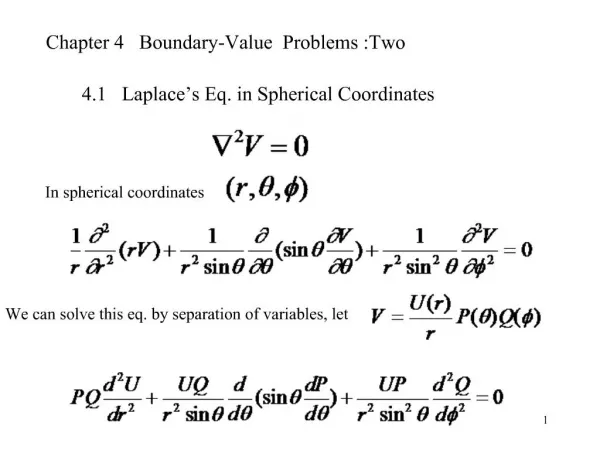
CONTINUOUS SOLUTION FOR BOUNDARY VALUE PROBLEMSON NON REGULAR GEOMETRY P. Venkataraman
TODAY’S PRESENTATION MOTIVATION BEZIER FUNCTIONAL REPRESENTATION EXAMPLE 1: POISSON’S EQUATION EXAMPLE 2: LAPLACE EQUATION EXAMPLE 3: NONLINEAR PDE CONCLUSION
Motivation I • Boundary Value Problems (BVP) on rectangular (regular) domain can be solved either by • Domain discretization techniques (finite element, finite volume, finite difference ), or, • Non-discretization techniques (meshless, analytical, using function approximation – adopted in this paper) • The advantage of the particular functional representation of this paper allows extraction of additional properties of the data that may not be obvious • Single solution over the domain • Continuous higher order derivatives • Analytical computation of incidental data based on the continiuos solution • Does not care if the system is linear, nonlinear, ordinary, partial, single, or coupled systems of differential equations
Motivation II This paper illustrates the solution of BVP on a nonrectangular (irregular) domains, using functional approximation through the Bezier functions (or Bernstein Polynomials) Currently such problems are only solved using domain discretization techniques • In essence, this is a meshless approach that provides all of the advantages mentioned in the previous slide and in addition the method is • Direct • Simple • Requires no transformation of the problem (strong form of BVP) • The solution (over the entire domain) is available in polynomial form (closed)
Motivation III The solution of the BVP is obtained using a standard least square error measure(or absolute error measure) in both the residuals and the boundary conditions Solution is determined at discrete points in the interior and the boundary The solution depends on the order of the function and therefore can only be considered approximate. However variation in the parameters of the method only changes the solution in a small way. Therefore, the solution can be considered robust Continuous solutions of the linear BVP over a nonrectangular domain are usually not available, as far as the author can ascertain. The challenge of a continuous solution to a general nonlinear BVP over the same region is also a state of the art
Bezier Function Representation 1 For this paper, the Bernstein basis representation of the Bezier function, using two parameters, (r, s) is Each Bi,j represents a set three values, defining a vertex location in three-dimensional Euclidean space. m is the order of the surface ( also the polynomial) in x- direction. n is the order of the surface ( also the polynomial) in the y – direction. Jm,i and Kn, j are the Bernstein basis or polynomial form. The use of the Bézier function guarantees the existence of a bounded real valued function (provided the vertices are bounded) The numerical optimizer will determine design variables that are bounded. Therefor an approximate solution to the BVP problem will always exist even if its quality is wanting.
Bezier Function Representation 2 We linearly relate the parameters r and s to the independent variables x and yWe take advantage of this transformation to generate the higher derivatives of the functions used in the BVP, and if necessary, for Neumann boundary conditions. A mixture of symbolic and numeric computation is used for computation, The formulation of the error is through symbolic calculation The minimization of the error is accomplished numerically The translation from symbolic to numeric objective function for the optimizer is done using a special built-in matlabFunction function. The solution was discovered through the unconstrained optimizer fminunc from the MATLAB Optimization Toolbox
Example 1: POISSON’S EQUATION 1 The first problem is the solution to Poisson’s equation over a circular domain Points used to generate the solution Points used to calculate residuals Points used to calculate boundary error
Example 1: POISSON’S EQUATION 2 Objective function : Number of Bézier points is 36 (for function of order 5). Number of points on the boundary (nB) was 21. Number of total points for the error in the residuals (nR) were 278. The problem has an analytical solution of second order
Example 1: POISSON’S EQUATION 3 Bezier Solution (5, 5) COMSOL Solution
Example 2: LAPLACE EQUATION 1 This example deals with Laplace equation over a five sided region There are 4 straight edges and 1 quarter circle The boundary conditions at the edges are also detailed on the figure For discontinuous solution (FEM), the temperatures at the intersection of the edges can have different temperatures on the two edges. That is different temperatures at the same point For continuous solution on the domain, the same point cannot have two different values – therefore solutions will violate discontinuous boundary conditions. The figure above indicates the modified boundary conditions
Example 2: LAPLACE EQUATION 2 m = 9, n = 9 Solution Bezier points (100) Residual points (260) Boundary points (50)
Example 2: LAPLACE EQUATION 3 COMSOL Solution Continuous Solution Residual Error Boundary Error
Example 3: A Nonlinear Equation 1 A nonlinear example on the same domain with same boundary conditions The only change required is to incorporate the new residual function Everything else remained the same – including the starting guesses and the optimizer. • Generally: • errors are bigger • more iterations • solution moves to a local minimum Objective function can be the least squared error in the residuals and the boundary conditions – OR –least sum of absolute error in the residuals and boundary conditions
Example 3: A Nonlinear Equation 2 No solution is available for comparison. Therefore two solutions are shown Final Solution Structured Initial Guess
Example 3: A Nonlinear Equation 3 Final Solution (structured) Final Solution Random Initial Guess Therefore we have a mesh free procedure to obtain a continuous solution to PDEs, on a non-rectangular domain, irrespective of the linear or nonlinear nature of the PDE.
Conclusions 1. The formulation is simple 2. The set up is direct 3. Meshless (no domain discretization) 4. Differential equations handled in original form 5. Exact derivatives in residual computation 6. Standard unconstrained optimizer 7. Procedure is independent of type or class of problems 8. A single continuous solution over the entire domain 9. Number of points for error computation is not important 10. A mix of symbolic and numeric computation for error control 11. The procedure provides decent approximate solutions for difficult BVP
Future Work 1. Incorporate analytical gradients because the formulation is symbolic to improve and speed convergence 2. To investigate separable solutions to take advantage of the excellent blending properties of the Bernstein basis 3. Reduce dimension of the problem through separable solutions 4. Extend these investigations to Inverse problems in non rectangular domains