Multiplexed Fluorescence Unmixing
Multiplexed Fluorescence Unmixing. Marina Alterman , Yoav Schechner. Technion , Israel. Aryeh Weiss. Bar- Ilan , Israel. Natural Linear Mixing. i. c. i. c. Raskar et al. 2006. i. c. ImageJ image sample collection. Natural Linear Mixing. ?. + noise. i. c. i. + noise.

Multiplexed Fluorescence Unmixing
E N D
Presentation Transcript
Multiplexed Fluorescence Unmixing Marina Alterman, YoavSchechner Technion, Israel Aryeh Weiss Bar-Ilan, Israel
Natural Linear Mixing i c i c Raskar et al. 2006. i c ImageJ image sample collection.
Natural Linear Mixing ? + noise i c i + noise c Raskar et al. 2006. i + noise How do you measure i? c ImageJ image sample collection.
a1 1 0 i 1 1 a = 0 1 1 i 2 2 a1 0 1 i 3 3 Single Source Excitation demultiplex Multiplexed Excitation i1 2 1 a1 1 3 i2 a2 2 1 3 i3 a3 3 Beam combiner 2
Why Multiplexing? Trivial Measurements Multiplexed Measurements i + noise SNR SNR Intensity vector Same acquisition time
i – single source intensities η - noise Multiplexing - Look closer Estimate c noti Xc i acquisition estimation Minimum W=?
Multiplexing: a=Wi, Mixing: i=Xc Common Approach This Work Acquired multiplexed intensities Single source intensities Concentrations ˆ ˆ ˆ ˆ c c i i a a Wi≠Wc Wi Wc Ndyes=3 Nsources=7 Nmeasure=3 size(i)=7 efficient acquisition Nmeasure=7 Alterman, Schechner & Weiss, Multiplexed Fluorescence Unmixing
Fluorescence Cell structure and processes Fluorescent Specimen Horse Dermal Fibroblast Cells Corn Grain Intestine Tissue Flea http://www.microscopyu.com/galleries/fluorescence, http://www.microscopy.fsu.edu/primer/techniques/fluorescence/fluorogallery.html
Linear Mixing i More molecules per pixel Brighter pixel c i c Molecules per pixel i = x∙c Alterman, Schechner & Weiss, Multiplexed Fluorescence Unmixing
Linear Mixing i {cd} i = x x ∙ ∙ ∙ x For each pixel: c c ∙ ∙ ∙ c 1 2 Ndyes 1 2 Ndyes vector of concentrations (spatial distribution) Alterman, Schechner & Weiss, Multiplexed Fluorescence Unmixing
Linear Mixing i i 1 2 s=1 s=2 {cd} {cd} For each pixel: i = x x ∙ ∙ ∙ x i = x x ∙ ∙ ∙ x i = x x ∙ ∙ ∙ x c c ∙ ∙ ∙ c 1 2 s 2,1 2,2 2,Ndyes 1,1 1,2 1,Ndyes s,1 s,2 s,Ndyes 1 2 Ndyes ∙ ∙ ∙ vector of concentrations (spatial distribution) vector of intensities Mixing matrix
Linear Mixing i i 1 2 s=1 s=2 {cd} {cd} For each pixel: vector of concentrations (spatial distribution) vector of intensities Mixing matrix
Fluorescent Microscope Intensity image e(λ) Emission Filter s = 1 s = 2 s = 3 e(λ) s = 4 Dichroic Mirror L2(λ) s = 5 Excitation Excitation Fluorescent Filter Sources λ λ λ 300 400 500 600 700 300 400 500 600 700 300 400 500 600 700 Specimen s: illumination sources Blue α(λ)
Fluorescent Microscope Intensity image (mixed) Intensity image e(λ) Unmixing required Emission Filter s = 1 s = 2 s = 3 e(λ) s = 4 Dichroic Mirror L2(λ) s = 5 Excitation Excitation Fluorescent Filter Sources λ λ λ 300 400 500 600 700 300 400 500 600 700 300 400 500 600 700 Specimen s: illumination sources Green Blue Cross-talk α(λ) Cross-talk
Unmix Fluorescent specimen Problem Definition Intensity image (mixed) + noise noise How to multiplex for least noisy unmixing? Alterman, Schechner & Weiss, Multiplexed Fluorescence Unmixing
Sum up the concepts Man made Nature Acquired multiplexed image intensities Single source Image intensities W X a i Concentrations multiplexing mixing c unmixing demultiplexing W-1 X-1 multiplexed unmixing Alterman, Schechner & Weiss, Multiplexed Fluorescence Unmixing
Look closer - again i – single source intensities η - noise Xc i Estimate c noti Alterman, Schechner & Weiss, Multiplexed Fluorescence Unmixing
Multiplexed Unmixing acquisition For each pixel i acquired measurements noise estimation a X W c WX is not square + = Weighted Least Squares Other estimators OR multiplexing matrix OR mixing matrix Minimum Variance in c W=?
Generalizations Minimum Var W=? η - noise Image intensities i =? var(η) =constant Details in the paper concentrations c =? var(η) =constant c =? var(η) ≠constant Alterman, Schechner & Weiss, Multiplexed Fluorescence Unmixing
Generalized Multiplex Gain What is the SNR gain for unmixing? Only Unmixing VS. Unmixing + Multiplexing Alterman, Schechner & Weiss, Multiplexed Fluorescence Unmixing
2.2 2 1.8 1.6 1.4 1.2 1 3 4 5 6 7 Nsources=Nmeasure Significance of the Model ˆ ˆ c GAINc ˆ ˆ c i i a a VS. Wi≠Wc Wi Wc Alterman, Schechner & Weiss, Multiplexed Fluorescence Unmixing
2.2 2 1.8 1.6 1.4 1.2 1 3 4 5 6 7 Nsources=Nmeasure Significance of the Model ˆ ˆ c GAINc i a Wc Alterman, Schechner & Weiss, Multiplexed Fluorescence Unmixing
Significance of the Model ˆ ˆ 2.2 c GAINc ˆ ˆ c i i a 2 a 1.8 1.6 Wi 1.4 1.2 1 Wc 3 4 5 6 7 GAIN < 1 Nsources=Nmeasure For specific 3 dyes, camera and filter characteristics
Natural Linear Mixing ? + noise i c i + noise c Raskar et al. 2006. i + noise c ImageJ image sample collection.
Multiplexed Unmixing Xc i Generalization of multiplexing theory The goal is unmixing SNR improvement Efficient Acquisition Exploit all available sources a X + = c η W Alterman, Schechner & Weiss, Multiplexed Fluorescence Unmixing