Download
1 / 13
260 likes | 805 Views
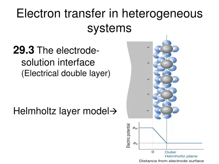
Electron transfer in heterogeneous systems. 29.3 The electrode-solution interface (Electrical double layer) Helmholtz layer model . Gouy-Chapman Model. This model explains why measurements of the dynamics of electrode processes are almost done using a large excess of supporting electrolyte.

E N D
Electron transfer in heterogeneous systems 29.3The electrode-solution interface (Electrical double layer) Helmholtz layer model
Gouy-Chapman Model • This model explains why measurements of the dynamics of electrode processes are almost done using a large excess of supporting electrolyte. ( Why??)
The Stern model of the electrode-solution interface • The Helmholtz model overemphasizes the rigidity of the local solution. • The Gouy-Chapman model underemphasizes the rigidity of local solution. • The improved version is the Stern model.
Outer potential • Inner potential • Surface potential • The potential difference between the points in the bulk metal (i.e. electrode) and the bulk solution is the Galvani potential difference which is the electrode potential discussed in chapter 10. The electric potential at the interface
The origin of the distance-independence of the outer potential
The connection between the Galvani potential difference and the electrode potential • Electrochemical potential (û) û = u + zFø • Discussions through half-reactions
29.4 The rate of charge transfer • Expressed through flux of products: the amount of material produced over a region of the electrode surface in an interval of time divided by the area of the region and the duration of time interval. • The rate laws Product flux = k [species] The rate of reduction of Ox, vox = kc[Ox] The rate of oxidation of Red, vRed = ka[Red] • Cathodic current density: jc = F kc[Ox] for Ox + e-→ Red ja = F ka[Red] for Red →Ox + e- the net current density is: j = ja – jc = F ka[Red] - F kc[Ox]
The activation Gibbs energy • Write the rate constant in the form suggested by activated complex theory: • Notably, the activation energies for the catholic abd anodic processes could be different!
The Butler-Volmer equationVariation of the Galvani potential difference across the electrode –solution interface
The parameter α is called the transient coefficient and lies in the range 0 to 1. Based on the above new expressions, the net current density can be expressed as:
The lower overpotential limit • The high overpotential limit