Download
1 / 17
180 likes | 336 Views
Precipitation studies with RADARS and use of WP/RASS By S.H. Damle. In precipitating conditions a vertically pointing Doppler Radar Effectively measures the apparent fall velocity of the falling hydrometers/snow particles The scattering in most cases is presumed to be Rayleigh

E N D
Precipitation studies with RADARS and use of WP/RASS By S.H. Damle
In precipitating conditions a vertically pointing Doppler Radar Effectively measures the apparent fall velocity of the falling hydrometers/snow particles • The scattering in most cases is presumed to be Rayleigh • The apparent/observed fall velocity deviates from true fall velocity because of • Ambient clear air velocity & turbulence • Pressure dependence of fall velocity • Deviations from the assumed Rayleigh scattering mechanism
The ambient clear air velocity & turbulence are the most important and must be known with reasonable accuracy/ confidence level to obtain the true fall velocities & other related parameters from the observed ‘apparent velocity • The classical work of Atlas and Srivastav (1973) shows that the clear air updrafts/downdrafts should preferably be measured with accuracies of 0.25 m/sec or better to obtain reasonable estimates of the rain related parameters
The conventional S/C/X band Radars can not quite measure the turbulent clear air motion – the scale sizes of turbulence to which they could respond being much smaller ~ λ /2 • In the absence of clear air velocity & turbulence , Roger used an empirical relation like to utilise radar precipitation data <Vf> = 2.65 Z ** 0.107 m/sec since <Vobs > = Vf - w where w is positive for upward air motion. • The Roger’s empirical relationship is approximate within ±1 m/sec
The advent of U/VHF Radars has now made possible direct measurement of ambient clear air updraft/downdraft and the turbulence. • Simultaneous measurement of clear air turbulent air velocities and the hydrometeor (apparent) fall velocities make possible the precipitation studies with these Radars.
The use of clear air wind profiler Radars • Typical clear air Radar operating frequencies 50, 400, 1380 MHz. • Clear air scattering mechanism – Bragg scatter - λ-1/3 dependence • Precipitation - Rayleigh scatter - λ-4 dependence • If one equates the expressions for the volume reflectivity for the two cases one obtains the relationship between the equivalent reflectivity factor Ze & the Cn2 Thus • dBZe = 10 log Ze = 10 {log 10 Cn2 + log λ11/3 +15.31} where λ is in meters and Ze is in mm6/m3 • Equation is valid for scattering from water droplets • Typical clear air Cn2 values are in the range of 10-15 to 10-18 m-2/3
From this table one can note • 50 MHz system would almost always measures the clear air velocity unless the precipitation rises beyond rain rate of few mm/hr • 1380 MHz profiler is sensitive to smallest of drizzle (rain rate 0.01mm/hr) and swamps the clear air signal. • This prompted research workers to use co-located or near by radars- one at 50 MHz and the other 915/1380 MHz for precipitation study. • The 400 MHz system case is intermediate between these two extremes and thus the 400 MHz profiler may be amenable to simultaneous observations of Bragg & Rayleigh scatter.
Relationships to dropsize distribution Z = ∫ D**6 * N (D) dD • The first task is to relate fall velocity with drop diameter Vf = a*D**b - unrealistic • GK data shows that fall speed approaches an asymptotic value of 9.2 m/sec for D > 6 mm • Atlas , Srivastava modification V=965-1030 exp (-6D) cm /sec, where D is in cm
Modified GK expression is valid near the ground • For higher heights Foote & Dutoit suggested a density correction factor to use them at higher heights Vh =vg (ρg/ρh)**0.4 • Thus if true fall velocity is calculated from radar observation, sample D values, within the limitation of spectral resolution, can be obtained for a given precipitation event.
Key factors to prepare algorithm development Location in the Doppler plane of the Bragg & Rayleigh scatter signal • Ralph’s prescriptions of velocity thresholds for Rayleigh scatter identification for rain • The Rayleigh scatter signal for height levels just below and above the zero degree isotherm level
The bright band signature - Large velocities just below freezing level heights and steep fall in the speed towards freezing level heights – indicative of presence of snow at/above freezing level - Absence of Bright Band – indicative of presence of super cooled water droplets above freezing levels • The (Doppler) velocity value in the case of snow/ice particulates is less than that of water droplets because of lower density of ice/snow compared to that of water
Signal flow in a profiler Objective Determination of noise power; Hildebrand/Sekhon algorithm • Obtain average noise power/bin ……… Pn & standard deviation ……σn For a given range bin • Subtract average noise power from spectral value • Identify clear air spectral peak • Identify precipitation spectra peak • Fit Gaussian curve for clear air spectra and estimate clear air velocity and spread • Deconvolve the ppt spectrum by clear air spectrum and obtain ppt spectral width
Observed Spectrum Deconvolution of Window function Find clear-air spectrum : St Fitting clear-air spectrum Find precipitation spectrum : SD Set initial precipitation spectrum Convolution : St * SD Comparison with observed spectrum Convergence decision Iteration Retrieval of raindrop size distribution
For lower rain rates it may be acceptable to fit Gaussian curve to ppt spectra and estimate apparent fall velocity and apparent spectral / observed width σtp**2 = σpo**2-σcl**2 • True fall velocity = observed velocity – clear air velocity • Calculate dBZ from estimated S/N
Illustration with common size distribution N(D) = N0 exp (-λD) V = 965 -1030 { (λ/(λ+6))} 7 cm /sec • With knowledge of λ and sample value of D as obtained earlier one may estimate N0 for every measurement height by relating to Z as indicated earlier • Variation of N0 and λ with height may provide by extrapolation estimation of expected distribution of ground • The knowledge of variation of the distribution with time could possibly correlated with cloud models to study the evolution.
Concluding Remarks Difficulties arise when • Separate Bragg and Rayleigh scatter peaks can not be identified in the spectrum The topic is of current research interest : April 2005 : JOAT • Use of iterative deconvolution. • Works with additional external constraints in the algorithm since iterative methods can lead to divergent solutions • Model spectra fitting is carried out using gamma distribution – 400 MHz • More work needed for the case when two distinct peaks can not be identified.