Source Detection I:Theory
Source Detection I:Theory. P. E. Freeman & V. Kashyap 3 rd X-ray Astronomy School 14 May 2003. The Challenge: Source Detection. What challenge??. (Granted, it does look easy here. This is a Hubble image of the globular cluster 47 Tuc, courtesy P. Edmonds.).

Source Detection I:Theory
E N D
Presentation Transcript
Source Detection I:Theory P. E. Freeman & V. Kashyap 3rd X-ray Astronomy School 14 May 2003
The Challenge: Source Detection What challenge?? (Granted, it does look easy here. This is a Hubble image of the globular cluster 47 Tuc, courtesy P. Edmonds.)
The Challenge: Source Detection It gets harder: not everything seen in this false-color Chandra image of the core for 47 Tuc is an X-ray source. (P. Edmonds) As seen in this ROSAT image of the Pleiades, the X-ray source detector must worry about high backgrounds and exposure variations (the edge of the circular field-of-view and the support-rib shadows). (V. Kashyap)
The Challenge: Source Detection • Sources may be easy to see in a typical Hubble image. However, detecting and characterizing them becomes increasingly difficult at higher energies. • Source data may consist of only a few counts, hence we must rely on the Poisson distribution when making statistical inferences. • Some spatially extended sources (e.g., supernova remnants) emit brightly at high energies and may overlap with point sources, making detection and characterization of the latter more difficult. • How a high-energy telescope blurs a point source (i.e., the telescope’s point-spread function) may be spatially non-uniform. • Is this a source, or a background fluctuation?
Detection Theory: the Short Form Note: the following statements are generic; they may or may not apply to the specific source detection algorithm of your choice. They are meant to build your intuition. • The Ingredient(s): a N-dimensional event list or binned “image.” (And an exposure map, knowledge of the PSF, etc., if appropriate.) • The Detection “Tool”: some function that is localized (i.e., non-zero only over some characteristic scale) within at least some subset of the dimensions. • The Hypotheses: M0: the data in a given pixel are (Poisson-)sampled from the background. M1: the data are a sum of samples from the background and an astronomical source.
The Five-Fold Path For a given source detection algorithm, an analyst might follow this five-fold path to source detection Nirvana: • Select an appropriate function scale, σ. (If one is attempting to detect a point source, this would be some encircled-energy radius of the PSF.) • Estimate the background amplitude, B. (In actuality, one would do this estimation for each image pixel-here, we narrow the problem to a single pixel.) • Determine the value of a selected model comparison test statistic, To. • Determine the significance, α: • Compare α to a pre-determined threshold significance value αo. If α < αo, the pixel is associated with a source!
Classic Detection: CELLDETECT • The Function(s): two box functions with unit amplitude, co-aligned and centroided at pixel (i,j). The number of counts within each box are Dd and Db. • The Determination of B: done by assuming (a) the truth of the alternative model, and (b) that the source is point-like: where α and β are the integrals of the PSF within each box, respectively. • The Model Comparison Test Statistic: the signal-to-noise ratio, or SNR: • Associating a Pixel with a Source: If SNR > SNRthr, accept the alternative model. • For more information: CIAO detect manual.
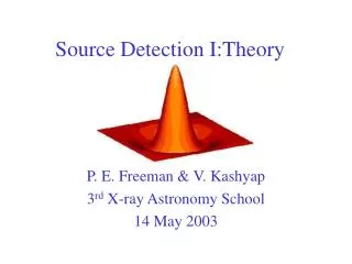
New Detection: WAVDETECT • The Function: the Marr, or “Mexican Hat” wavelet, W(σ) (above, right), which is non-zero within a circle of radius 5σ from the centroid. • The Determination of B: done by determining the average number of counts per pixel in the wavelet negative annulus (below, right), while using it as a weighting function; done iteratively, with source counts removed from the field until the background estimate stabilizes. • The Model Comparison Test Statistic: To = Co = Σi’ Σj’ W i-i’,j-j’ D i’j’ • Associating a Pixel with a Source: if α =Co dC p(C|2πσ2B) < αo accept. A typical choice for the threshold is 1/P, where P is the number of pixels examined in the image; it thus corresponds to a number of false pixels. See Freeman et al. 2002, ApJS 138, 185 for more details.
Why Mexican-Hat Wavelets? • The Gaussian-like positive kernel has a shape similar to canonical point-spread functions (PSFs). • The function is localized in both the spatial and Fourier domains; a dyadic (factors of two) sequence of scales is sufficient to sample the frequency domain. • It has two “vanishing moments”: the correlation of MH with constant and linear functions is zero. It thus “annihilates” the contribution of a spatially constant or linear background to the correlation coefficients.
Potholes on the Five-Fold Path • PSFs in the X-ray regime are spatially varying (which partially motivates the multi-scale approach to source detection; the other major motivation is the study of extended sources, e.g., SNRs, hot gas in clusters). • The optimal determination of B from raw data consisting of source and background counts is an unsurmounted statistical challenge. • The cosmic background is not necessarily spatially constant! • The probability sampling distributions (PSDs) from which observed values of T are sampled generally cannot be represented analytically, except asymptotically in the high-counts limit; simulations are needed. • There is no model comparison test statistic T that has been proven to be “most powerful”…and test power is extremely difficult to compute. • And exposure maps, vignetting, etc.: Vinay speaks of these. • Below, I expand on some of these issues…
Pothole: Spatially Varying PSFs A point source observed on-axis (center) with an X-ray telescope will be more sharply in focus than a source observed off-axis (outer eight panels), in large part because the counts-recording instruments are flat. Sources detected using a cell or wavelet of one scale may not be detected at another scale: a multi-scale approach is necessary for robust detection!
Pothole: Background Determination Strong source biases background in ring around it: • In theory, can model cosmic+particle background, but not easily done. • Estimated from raw data. How to do? • If one uses PSF information, one must make assumptions of spectral form (since width varies as function of energy); also, bad for detecting extended sources. • WAVDETECT computes backgrounds at each scale, and combines them; accurate enough for source detection, but systematic rings (top right) and bumps (bottom right) make final result not necessarily quanitatively accurate. Large-scale source biases background at source location:
Pothole: Spatially Varying Backgrounds Nearby regions of dense gas/dust can absorb the cosmic background (e.g., from AGNs), creating X-ray “shadows” such as that observed in the Pleiades. (Nearby emission in the hot local bubble means that we still see background photons in shadowed regions.)
Pothole: Computation of Significance • In the high-count limit, p(C|q = 2πB2) tends to a zero-mean Gaussian distribution of width σ = q1/2. • Elsewhere, p(C|q) is determined via simulations. (At right, a sample PSD at low counts from Damiani et al. 1997.)
Pothole: Computation of Significance The picture to the right shows the significance (from simulations) as a function of q and C (to the left of the cusp) or C/sqrt(q) (to the right of the cusp). The contours are 0.1 (bottom) to 10-7 (top). This figure demonstrates that a relatively smooth distribution (asymptotically Gaussian, at high q) becomes very messy at low q, and shows that simulations are required. The low q limit is important for Chandra, whose the smaller field of view greatly reduces the number of cosmic background events per pixel per second, relative to ROSAT.
Pothole: Type II Error • The Type II error is nearly impossible to compute for current source detection algorithms because of the fuzzy way the problem is stated: the alternate hypothesis is that “pixel (i,j) includes some number of source counts.” • Computed instead is the “detection efficiency”: how often does the algorithm detection a source of strength x, at off-axis location y, when the background is z… • Unlike Type I error, detection efficiency is instrument-specific. • Depends on scale sizes, background, amplitude, extent, spectrum, and off-axis angle, in addition to the details of the exposure at the source location. • A related topic: upper limits (“I don’t detect a source at (i,j). How strong could an underlying source be and still not be detected?”). Rarely analytically computable, it can be read off from detection efficiencies, if those have been computed.

