Download
1 / 14
140 likes | 262 Views
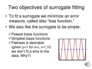
The two objectives of surrogate fitting. When we fit a surrogate we would like some error to be minimal. The general term of the quantity we minimize is “loss function.” We would also like the surrogate to be simple in some sense Fewest basis functions Simplest basis functions

E N D
The two objectives of surrogate fitting • When we fit a surrogate we would like some error to be minimal. The general term of the quantity we minimize is “loss function.” • We would also like the surrogate to be simple in some sense • Fewest basis functions • Simplest basis functions • Flatness (give y=1 for x=i, i=1,10 we could fit a sine to the data. Why don’t we?)
Support Vector Regression • Interesting history: • Generalized Portrait algorithm (Vapnik and Lerner, 1963, Vapnik and Chervonekis (1963, 1974). Russia. Properties of learning machines which enable them to generalize well to unseen data • Support Vector Machine. Bell Labs. Vapnik and coworkers (1992 on). Optical character recognition and object recognition. • Application to regression since 1997. • First part of lecture based on Smola and Scholkopf (2004), see reference material.
Support vector classifier • In engineering optimization community, support vector machines have been promoted as classifiers for feasibility • Notably the work of Sammy Missoum of University of Arizona. • Anirban Basudhar and SamyMissoum. ”An improved adaptive sampling scheme for the construction of explicit boundaries”.Structural and Multidisciplinary Optimization
Basic idea • We do not care about error below epsilon, but we care about magnitude of polynomial coefficients
Linear approximation • If noise limit is known and function is exactly linear • Can define following optimization problem • Objective function reflects “flatness” • Problem may not be feasible
“Soft” formulation • Primal problem • Second term in objective corresponds to -insensitive loss function
Optimality criteria • Lagrangian function • Karush-Kuhn-Tucker conditions and
Dual formulation • Substitute from KKT to Lagrangian, get dual • Also • Active constraints • Sparse approximation!
General case (Girosi-see reference) • Expansion in terms of base functions • Cost function balances error and “flatness” • Error cost function • Smoothness or flatness cost
Solution of variational problem • Independent of smoothness coefficients • Where symmetric kernel is • For -insensitive error cost function
Example • Find Young’s modulus from strain-stress measurements ε=[1,2,3,4] milistrains σ=[9,22,36,39] ksi. • Regression solution E=10.567 Msi • With third point identified as outlier, get E=9.95 Msi
An SVR solution eps=[ 1 2 3 4]; sig=[9 22 36 39]; slack=5; c=100; err=eps*E-sig; loss=max(abs(err)-slack,0); object=c*sum(loss)+0.5*E^2; End [E,fval]=fminsearch(@svyoung,xo) E =10.3333 fval =53.3890 err =1.3333 -1.3333 -5.0000 2.3334